
5.5.5: Alongshore balance-longshore current
- Page ID
- 16330

\( \newcommand{\vecs}[1]{\overset { \scriptstyle \rightharpoonup} {\mathbf{#1}} } \)
\( \newcommand{\vecd}[1]{\overset{-\!-\!\rightharpoonup}{\vphantom{a}\smash {#1}}} \)
\( \newcommand{\id}{\mathrm{id}}\) \( \newcommand{\Span}{\mathrm{span}}\)
( \newcommand{\kernel}{\mathrm{null}\,}\) \( \newcommand{\range}{\mathrm{range}\,}\)
\( \newcommand{\RealPart}{\mathrm{Re}}\) \( \newcommand{\ImaginaryPart}{\mathrm{Im}}\)
\( \newcommand{\Argument}{\mathrm{Arg}}\) \( \newcommand{\norm}[1]{\| #1 \|}\)
\( \newcommand{\inner}[2]{\langle #1, #2 \rangle}\)
\( \newcommand{\Span}{\mathrm{span}}\)
\( \newcommand{\id}{\mathrm{id}}\)
\( \newcommand{\Span}{\mathrm{span}}\)
\( \newcommand{\kernel}{\mathrm{null}\,}\)
\( \newcommand{\range}{\mathrm{range}\,}\)
\( \newcommand{\RealPart}{\mathrm{Re}}\)
\( \newcommand{\ImaginaryPart}{\mathrm{Im}}\)
\( \newcommand{\Argument}{\mathrm{Arg}}\)
\( \newcommand{\norm}[1]{\| #1 \|}\)
\( \newcommand{\inner}[2]{\langle #1, #2 \rangle}\)
\( \newcommand{\Span}{\mathrm{span}}\) \( \newcommand{\AA}{\unicode[.8,0]{x212B}}\)
\( \newcommand{\vectorA}[1]{\vec{#1}} % arrow\)
\( \newcommand{\vectorAt}[1]{\vec{\text{#1}}} % arrow\)
\( \newcommand{\vectorB}[1]{\overset { \scriptstyle \rightharpoonup} {\mathbf{#1}} } \)
\( \newcommand{\vectorC}[1]{\textbf{#1}} \)
\( \newcommand{\vectorD}[1]{\overrightarrow{#1}} \)
\( \newcommand{\vectorDt}[1]{\overrightarrow{\text{#1}}} \)
\( \newcommand{\vectE}[1]{\overset{-\!-\!\rightharpoonup}{\vphantom{a}\smash{\mathbf {#1}}}} \)
\( \newcommand{\vecs}[1]{\overset { \scriptstyle \rightharpoonup} {\mathbf{#1}} } \)
\( \newcommand{\vecd}[1]{\overset{-\!-\!\rightharpoonup}{\vphantom{a}\smash {#1}}} \)
\(\newcommand{\avec}{\mathbf a}\) \(\newcommand{\bvec}{\mathbf b}\) \(\newcommand{\cvec}{\mathbf c}\) \(\newcommand{\dvec}{\mathbf d}\) \(\newcommand{\dtil}{\widetilde{\mathbf d}}\) \(\newcommand{\evec}{\mathbf e}\) \(\newcommand{\fvec}{\mathbf f}\) \(\newcommand{\nvec}{\mathbf n}\) \(\newcommand{\pvec}{\mathbf p}\) \(\newcommand{\qvec}{\mathbf q}\) \(\newcommand{\svec}{\mathbf s}\) \(\newcommand{\tvec}{\mathbf t}\) \(\newcommand{\uvec}{\mathbf u}\) \(\newcommand{\vvec}{\mathbf v}\) \(\newcommand{\wvec}{\mathbf w}\) \(\newcommand{\xvec}{\mathbf x}\) \(\newcommand{\yvec}{\mathbf y}\) \(\newcommand{\zvec}{\mathbf z}\) \(\newcommand{\rvec}{\mathbf r}\) \(\newcommand{\mvec}{\mathbf m}\) \(\newcommand{\zerovec}{\mathbf 0}\) \(\newcommand{\onevec}{\mathbf 1}\) \(\newcommand{\real}{\mathbb R}\) \(\newcommand{\twovec}[2]{\left[\begin{array}{r}#1 \\ #2 \end{array}\right]}\) \(\newcommand{\ctwovec}[2]{\left[\begin{array}{c}#1 \\ #2 \end{array}\right]}\) \(\newcommand{\threevec}[3]{\left[\begin{array}{r}#1 \\ #2 \\ #3 \end{array}\right]}\) \(\newcommand{\cthreevec}[3]{\left[\begin{array}{c}#1 \\ #2 \\ #3 \end{array}\right]}\) \(\newcommand{\fourvec}[4]{\left[\begin{array}{r}#1 \\ #2 \\ #3 \\ #4 \end{array}\right]}\) \(\newcommand{\cfourvec}[4]{\left[\begin{array}{c}#1 \\ #2 \\ #3 \\ #4 \end{array}\right]}\) \(\newcommand{\fivevec}[5]{\left[\begin{array}{r}#1 \\ #2 \\ #3 \\ #4 \\ #5 \\ \end{array}\right]}\) \(\newcommand{\cfivevec}[5]{\left[\begin{array}{c}#1 \\ #2 \\ #3 \\ #4 \\ #5 \\ \end{array}\right]}\) \(\newcommand{\mattwo}[4]{\left[\begin{array}{rr}#1 \amp #2 \\ #3 \amp #4 \\ \end{array}\right]}\) \(\newcommand{\laspan}[1]{\text{Span}\{#1\}}\) \(\newcommand{\bcal}{\cal B}\) \(\newcommand{\ccal}{\cal C}\) \(\newcommand{\scal}{\cal S}\) \(\newcommand{\wcal}{\cal W}\) \(\newcommand{\ecal}{\cal E}\) \(\newcommand{\coords}[2]{\left\{#1\right\}_{#2}}\) \(\newcommand{\gray}[1]{\color{gray}{#1}}\) \(\newcommand{\lgray}[1]{\color{lightgray}{#1}}\) \(\newcommand{\rank}{\operatorname{rank}}\) \(\newcommand{\row}{\text{Row}}\) \(\newcommand{\col}{\text{Col}}\) \(\renewcommand{\row}{\text{Row}}\) \(\newcommand{\nul}{\text{Nul}}\) \(\newcommand{\var}{\text{Var}}\) \(\newcommand{\corr}{\text{corr}}\) \(\newcommand{\len}[1]{\left|#1\right|}\) \(\newcommand{\bbar}{\overline{\bvec}}\) \(\newcommand{\bhat}{\widehat{\bvec}}\) \(\newcommand{\bperp}{\bvec^\perp}\) \(\newcommand{\xhat}{\widehat{\xvec}}\) \(\newcommand{\vhat}{\widehat{\vvec}}\) \(\newcommand{\uhat}{\widehat{\uvec}}\) \(\newcommand{\what}{\widehat{\wvec}}\) \(\newcommand{\Sighat}{\widehat{\Sigma}}\) \(\newcommand{\lt}{<}\) \(\newcommand{\gt}{>}\) \(\newcommand{\amp}{&}\) \(\definecolor{fillinmathshade}{gray}{0.9}\)In the alongshore direction the transfer of momentum from the wave motion to the mean flow gives rise to a longshore current. Note that besides this wave-induced (due to wave dissipation in the breaker zone) current, also tidal and wind forces can generate a current along the coast. These are discussed in Sect. 5.6 and Sect. 5.7.2.
The longshore current (velocity magnitude and cross-shore distribution) is an import- ant input parameter in longshore sediment transport computations.
Alongshore momentum balance (straight, parallel depth contours)
We consider again the 2D situation (see Fig. 5.4) of a long-crested wave obliquely incident to an alongshore uniform coast (\(\theta = \varphi\) and all \(y\)-derivatives are zero). The cross-shore rate of variation of the shear component of the radiation stress \(S_{yx}\) acts as a driving force (Eq. 5.5.3.4). In the cross-shore direction the balancing force was supplied by a hydraulic pressure gradient. However, for an infinitely long uninterrupted coast- line, no such hydraulic pressure gradient can develop in the alongshore direction. The counterforce restoring equilibrium therefore must be supplied by bed shear stresses that develop when a longshore current is generated. The bottom shear stress restrains the current and is non-zero only in the presence of a current. Note that in the cross-shore direction the bed shear stress associated with the mean current was assumed small as compared to the pressure force.
We only consider the stationary situation. The alongshore component of the momentum balance for a steady state and alongshore uniformity can be written as:
\[F_y = -\dfrac{dS_{yx}}{dx} = \bar{\tau}_{b,y}\label{eq5.5.5.1}\]
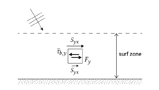
The balance between the driving force and the resisting or retarding force is shown in Fig. 5.36.
Wave force in alongshore uniform situation
Let us first assess \(F_y = -dS_{yx}/dx\) in deeper water, i.e. outside the breaker zone. In Sect. 5.5.2 we found \(S_{yx} = En \sin \varphi \cos \varphi \). The wave angle changes as a function of \(x\), but does not vary with \(y\). The latter leads to Snell’s law for regular waves (Eq. 5.2.3.1): \(\sin \varphi /c\) = constant. Conservation of energy (Eq. 5.2.1.2) requires \(d(Ec_g \cos \varphi)/dx = -D_w\) under the present assumptions. For linear waves we can now write the wave force Eq. 5.5.3.4 as:
\[F_y = -\dfrac{dS_{yx}}{dx} = -\dfrac{\sin \varphi}{c} \dfrac{d}{dx} Ec_g \cos \varphi = \dfrac{D_w}{c_0} \sin \varphi_0 \label{eq5.5.5.2}\]
Apparently the alongshore driving force is a function of the dissipation of the wave energy. Outside the surf zone the dissipation of wave energy can be neglected and hence the energy flux \(Ec_g = (Ec_g \cos \varphi, Ec_g \sin \varphi)\) is constant. We have in the absence of dissipation: \(S_{yx}\) and \(F_y = 0\). So although outside the surf zone the wave conditions change with \(x\) (wave height due to shoaling; wave direction due to refraction), the radiation shear stress is constant. Therefore, since the alongshore forcing is only present when the waves are breaking, the longshore current is confined to the surf zone (see also Intermezzo 5.6).
The finding that a mean current is only driven in the case of energy dissipation is universally valid, also in less simplified situations. The wave force consists of two parts:
- A part in the wave propagation direction that is related to the energy dissipation. This term is concentrated near the water surface where the dissipation actually takes place. This \(D/c\) part is rotational and can therefore induce mean currents or circulation currents in the case of a closed boundary. It is a result of the vorticity generated by wave breaking and stems from the effect of both velocity and pressure variation on the momentum flux;
- An irrotational part that is depth-invariant. This implies that there is no vertical imbalance. Thus, this part can be balanced by set-up and set down without driving currents. It only affects the wave-induced current indirectly, through its effect on the mean depth. In the surf zone the latter influence on the mean current is small compared with that of the dissipation.
Analytical model for alongshore wave force in the surf zone
To find an easy analytical expression for the longshore current we assume again the simple model for wave dissipation due to breaking that relates the wave height to the local water depth: \(H =\gamma h\) for every water depth in the surf zone. An alternative would be solving the energy balance numerically. The analytical expression is calculated from the dissipation model and Snell’s law:
\[F_y = -\dfrac{\sin \varphi}{c} \dfrac{d}{dx} Ec_g \cos \varphi = -\dfrac{\sin \varphi_0}{c_0} \dfrac{d}{dx} 1/8 \rho g \gamma^2 h^2 c_g \cos \varphi\]
In shallow water \(c_g = c = \sqrt{gh}\) and since due to refraction \(\varphi\) is small (generally around 10° to 15°) we assume \(\cos \varphi \approx 1\). We now have:
\[F_y \approx -\dfrac{\sin \varphi_0}{c_0} 1/8 \rho g^{3/2} \gamma^2 \dfrac{d}{dx} h^{5/2} = -\dfrac{5}{16} \dfrac{\sin \varphi_0}{c_0} \rho (gh)^{3/2} \gamma^2 \dfrac{dh}{dx}\]
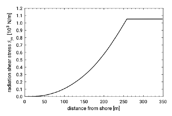
As mentioned above the radiation shear stress \(S_{yx}\) is constant seaward of the border of the breaker zone (thus the wave force is zero). It decreases inside the breaker zone to zero at the waterline (see Fig. 5.37).
For many day to day wave conditions, this gradient in \(S_{yx}\) causes alongshore stresses (forces) which are in the same order of magnitude as the bottom shear stress in rivers: in the order of \(1\ N/m^2\) to \(10\ N/m^2\). The cross-shore gradient in the alongshore radiation stress \(S_{yx}\) is therefore an important driving force in the littoral zone.
Quadratic friction law for bed shear stress
The next step is the formulation of the bed shear stress. In Sect. 5.4.3 we have already discussed the quadratic friction law for wave and current only situations. For currents the turbulence is present in the entire water column. The turbulence due to waves is present in the wave boundary layer only and significantly increases the bed shear stress. This is not only due to the significant increase in friction factors but due to the velocity being generally higher in the wave motion. For the vertical profile of the longshore current we need a quadratic resistance law of combined current and wave action. Such a law is non-trivial since:
- Due to the quadratic friction law the addition of the effects of waves and current is non-linear. Due to the non-linear addition, the combined shear stress averaged over the wave period is generally larger than the linear summation of the current only and wave only bed shear stress;
- The waves and currents may not have the same direction. The waves are incident with a certain angle whereas the longshore current is parallel to the coast. As a result the direction and magnitude of the bed-shear stress during the wave cycle varies continuously. The time-mean bed shear stress depends on the angle between the waves and current;
- As discussed earlier, for currents the turbulence is present in the entire water column and for waves in the wave boundary layer only. It therefore makes sense to relate the bed shear stress due to currents to a depth-mean velocity and due to waves to the free-stream velocity outside the wave boundary layer. The velocity at which height should be chosen for the combined wave current motion?
- Note that the above descriptions deal with the time-averaged bottom shear stress; they disregard the momentary (or intra-wave) shear stresses that may occur within the wave period. This seems reasonable when determining the wave- induced currents. However, the intra-wave velocity fluctuations may be import- ant for the net (wave-averaged) sediment transport (see also Chs. 6 and 7).
For the reasons mentioned above many different models exist for the bed shear stress under waves and currents. Depending on the model, the relative contributions of waves and currents to the bed shear stress vary. Some models describe the time-averaged bed shear stress, others the instantaneous bed shear stress. The description of the sediment transport requires an accurate (intra-wave or time-averaged, depending on the sediment transport model) bed shear stress. Therefore in Sect. 6.5 the bed shear stress is treated in more detail.
For the determination of the time-averaged bed shear stress in the alongshore direction, necessary to compute the longshore current, we take a fairly simple approach:
- The wave motion is described by shallow water theory (constant orbital amplitude outside the wave boundary layer);
- The angle of incidence is very small, such that for the wave motion \((u_x, u_y) = (\hat{u} \cos \omega t, 0)\);
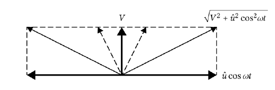
- The bed friction vector is related to the depth-averaged velocity vector. The latter is the sum of the depth-averaged longshore current velocity and the wave orbital motion: \(\vec{u} = (\hat{u} \cos \omega t, V)\), see Fig. 5.38;
-
The time-varying bed friction is written as:
\[\vec{\tau}_b = \rho c_f |\vec{u}| \vec{u}\] - The enhancement of the friction factor (compared to a current only situation) due to the small height of the wave boundary layer as compared to the current boundary layer is not further specified.
In the cross-shore direction, the time-averaged (not the instantaneous) bed shear stress is zero. With the above approximations, the time-averaged bed shear stress in the alongshore direction reads:
\[\bar{\tau}_{b,y} = \overline{\rho c_f |\vec{u}| V} = \rho c_f \sqrt{V^2 + \hat{u}^2 \cos^2 \omega t} V\]
If we further assume that \(V \ll \hat{u}\) this can be simplified to:
\[\bar{\tau}_{b,y} = \dfrac{2}{\pi} \rho c_f \hat{u} V\]
With \(\hat{u}\) in shallow water given by Eq. 5.4.1.2 and with a constant ratio of wave height over water depth across the entire surf zone we find:
\[\bar{\tau}_{b,y} = \dfrac{1}{\pi} \rho c_f \sqrt{gh} \dfrac{H}{h} V \label{eq5.5.5.8}\]
Analytical model for longshore current (no lateral dispersion)
For steady conditions the alongshore velocity follows from the balance between the driving force and the resisting friction force (Eq. \(\ref{eq5.5.5.1}\)). This yields with Eq. \(\ref{eq5.5.5.2}\)) and Eq. \(\ref{eq5.5.5.8}\)):
\[\dfrac{D_w}{c_0} \sin \varphi_0 = \dfrac{1}{\pi} \rho c_f \sqrt{gh} \dfrac{H}{h} V \Leftrightarrow V(x) = \dfrac{\pi}{c_f \rho g \sqrt{g}} \dfrac{\sin \varphi_0}{c_0} \dfrac{D_w (x)}{H(x)} \sqrt{h(x)}\]
The magnitude of the depth-averaged longshore current velocity varies in the surf zone as a function of the dissipation, wave height and water depth. The dissipation and wave heights can be modelled using a wave model (with roller model). In our simple dissipation model \(\gamma = H/h\) = constant and we can write the force balance Eq. \(\ref{eq5.5.5.1}\) as:
\[-\dfrac{5}{16} \dfrac{\sin \varphi_0}{c_0} \rho (gh)^{3/2} \gamma^2 \dfrac{dh}{dx} = \dfrac{1}{\pi} \rho c_f \sqrt{gh\gamma V}\]
which leads to:
\[V(x) = -\dfrac{5}{16} \pi \dfrac{\gamma}{c_f} g \dfrac{\sin \varphi_0}{c_0} h \dfrac{dh}{dx}\]
For a constant beach slop \(\tan \alpha = -d h_0/dx\) and for \(dh/dx \approx dh_0/dx\), the current velocity is proportional to the depth with a maximum at the breaker line (where \(h = h_b\)):
\[V(x) = \dfrac{5}{16} \pi \dfrac{H_b}{c_f} g \dfrac{\sin \varphi_0}{c_0} \dfrac{h}{h_b} \tan \alpha \label{eq5.5.5.12}\]
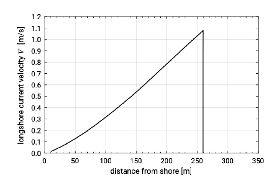
A longshore current profile according to Eq. \(\ref{eq5.5.5.12}\) is shown in Fig. 5.39. The larger the wave height \(H_b\) at breaking, the larger the maximum longshore current velocity and the wider the littoral zone; a factor 2 larger wave height, would then result in a factor 8 larger discharge in the surf zone. Eq. \(\ref{eq5.5.5.12}\) also allows us to get an idea of the effect of the beach slope \(\tan \alpha\). A steeper slope, on the one hand, results in (linearly) higher velocities. On the other hand the width of the surf zone becomes linearly smaller. The discharge through the entire surf zone is then constant to a first approximation (we have amongst others neglected the effect of the beach slope on the breaking parameter, Sect. 5.2.5). If the wave angle is small, the longshore current velocity at a specific water depth within the surf zone, becomes a linear function of \(\varphi_0\) (since: \(\sin \varphi_0 = \varphi_0\) for small \(\varphi_0\)).
Turbulent forces redistributing momentum
So far, the effect of lateral dispersion of momentum by turbulence has been ignored. Including turbulence in the momentum equation tends to smooth out velocity gradients (including the unrealistic velocity gradient at the breaker point).
Let us first look at turbulence and turbulence modelling in a bit more detail. In Sect. 5.4.3, the total velocity vector was said to be composed of a mean, a wave and a turbulent part. The turbulent shear stress was subsequently defined as the stress introduced when averaging over the turbulent motion. In analogy with the modelling of viscous stresses, in a turbulent flow the shear stress is generally related to velocity gradients through a turbulent or eddy viscosity \(v_T\). The molecular viscosity \(v\) seems to make water sticky and resist flowing and may be thought of as a measure of viscous fluid friction. Similarly \(v_T\) is a measure of turbulent fluid friction (in coastal waters \(v_T \gg v\)). The eddy viscosity \(v_T\) [\(m^2/s\)] depends on a characteristic spatial scale and on a characteristic velocity. In the littoral zone, both are related to the wave motion. The wave orbital motion, for instance, can be regarded as a measure for the characteristic velocity. For vertical mixing, the characteristic (mixing) length is the depth. Horizontal mixing is not restricted by water depth. For that reason, in nearshore modelling the horizontal eddy viscosity \(v_T, H\) is often taken much larger than \(v_T\) for vertical mixing. Typical values for the eddy viscosity \(v_T\) are \(10^{-2} m^2/s\).
We have seen that the driving force for the longshore current is \(\partial S_{yx} \partial x\). The shear component of the radiation stress \(S_{yx}\) was defined through Eq. 5.5.2.5, in which the velocity components are due to the orbital motion. In analogy with Eq. 5.5.2.5 we can write for the turbulent force:
\[S_{yx}' = \overline{\int_{-k_0}^{\eta} (\rho u_y' u_x') dz}\]
where the overbar now represents averaging over the turbulent motion (indicated with primes). This shear stress or friction force per unit surface area, acts on a surface parallel to the coast. It can be modelled as:
\[S_{yx}' \cong h \rho v_{T, H} \dfrac{dV}{dx}\]
The eddy viscosity \(v_T\) [\(m^2/s\)] is also referred to as horizontal diffusivity.
The momentum equation in the alongshore direction now reads:
\[\dfrac{D_w}{c_0} \sin \varphi_0 + \dfrac{d}{dx} \left (h \rho v_{T, H} \dfrac{dV}{dx} \right ) = \bar{\tau}_{b, y}\]
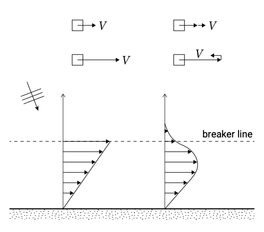
The effect of turbulent forces, smoothing the longshore current profile, is indicated in Fig. 5.40. Since the largest velocity gradient occurs at the breaker line, the maximum transfer of horizontal momentum will occur here. This leads to a reduction in the maximum velocity, a landward shift of the position of maximum velocity and to a situation where also outside the breaker zone longshore current velocities occur. The cross-shore distribution of the eddy viscosity now also determines the velocity distribution.
Roller momentum
Section 5.5.4 discussed that the measured onset of set-up occurs closer to the shore than predicted. This spatial lag was attributed to the roller momentum that had not been taken into account. Similarly longshore current velocity profiles show an onshore shift in the maximum longshore current velocity. This can be modelled by including the roller contribution in the alongshore momentum equation.
Irregular waves
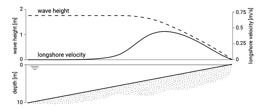
Until now we have only considered regular waves. In reality, of course, waves are irregular and there is no sharply defined breaker line. The effect of wave irregularity is therefore to smooth out the velocity distribution, very similar to the effect of turbulence, giving a wider and less sharply peaked velocity distribution. This is also illustrated in Fig. 5.41, which shows the output of a computation with the computer model Unibest-CL+.
Profile with breaker bar
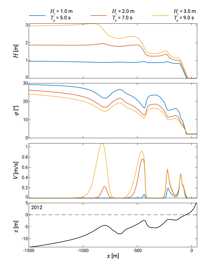
If we have a coastal profile with a breaker bar, then the determination of the velocity distribution gets more complicated. In a simplified approach, we can distinguish between a breaker zone at the seaward side of the breaker bar (if waves indeed break at the corresponding water depths) and a breaker zone near the shoreline where the remaining wave energy is dissipated. This simplification would lead to a zero long- shore current velocity in the deeper section between both breaker zones. Also in such a situation, both lateral transfer of horizontal momentum and the irregularity of the waves will smooth out the velocity distribution. An example of the longshore current distribution is given in Fig. 5.42. Wave breaking tends to concentrate on the bars and at these locations a longshore current is driven. For the highest wave condition, wave breaking already occurs at the outermost bar, whereas for the lowest wave condition wave breaking occurs only at the innermost bar and close to the shoreline.