5.5.6: Vertical structure of the wave-induced currents
- Page ID
- 16331
\( \newcommand{\vecs}[1]{\overset { \scriptstyle \rightharpoonup} {\mathbf{#1}} } \)
\( \newcommand{\vecd}[1]{\overset{-\!-\!\rightharpoonup}{\vphantom{a}\smash {#1}}} \)
\( \newcommand{\id}{\mathrm{id}}\) \( \newcommand{\Span}{\mathrm{span}}\)
( \newcommand{\kernel}{\mathrm{null}\,}\) \( \newcommand{\range}{\mathrm{range}\,}\)
\( \newcommand{\RealPart}{\mathrm{Re}}\) \( \newcommand{\ImaginaryPart}{\mathrm{Im}}\)
\( \newcommand{\Argument}{\mathrm{Arg}}\) \( \newcommand{\norm}[1]{\| #1 \|}\)
\( \newcommand{\inner}[2]{\langle #1, #2 \rangle}\)
\( \newcommand{\Span}{\mathrm{span}}\)
\( \newcommand{\id}{\mathrm{id}}\)
\( \newcommand{\Span}{\mathrm{span}}\)
\( \newcommand{\kernel}{\mathrm{null}\,}\)
\( \newcommand{\range}{\mathrm{range}\,}\)
\( \newcommand{\RealPart}{\mathrm{Re}}\)
\( \newcommand{\ImaginaryPart}{\mathrm{Im}}\)
\( \newcommand{\Argument}{\mathrm{Arg}}\)
\( \newcommand{\norm}[1]{\| #1 \|}\)
\( \newcommand{\inner}[2]{\langle #1, #2 \rangle}\)
\( \newcommand{\Span}{\mathrm{span}}\) \( \newcommand{\AA}{\unicode[.8,0]{x212B}}\)
\( \newcommand{\vectorA}[1]{\vec{#1}} % arrow\)
\( \newcommand{\vectorAt}[1]{\vec{\text{#1}}} % arrow\)
\( \newcommand{\vectorB}[1]{\overset { \scriptstyle \rightharpoonup} {\mathbf{#1}} } \)
\( \newcommand{\vectorC}[1]{\textbf{#1}} \)
\( \newcommand{\vectorD}[1]{\overrightarrow{#1}} \)
\( \newcommand{\vectorDt}[1]{\overrightarrow{\text{#1}}} \)
\( \newcommand{\vectE}[1]{\overset{-\!-\!\rightharpoonup}{\vphantom{a}\smash{\mathbf {#1}}}} \)
\( \newcommand{\vecs}[1]{\overset { \scriptstyle \rightharpoonup} {\mathbf{#1}} } \)
\( \newcommand{\vecd}[1]{\overset{-\!-\!\rightharpoonup}{\vphantom{a}\smash {#1}}} \)
\(\newcommand{\avec}{\mathbf a}\) \(\newcommand{\bvec}{\mathbf b}\) \(\newcommand{\cvec}{\mathbf c}\) \(\newcommand{\dvec}{\mathbf d}\) \(\newcommand{\dtil}{\widetilde{\mathbf d}}\) \(\newcommand{\evec}{\mathbf e}\) \(\newcommand{\fvec}{\mathbf f}\) \(\newcommand{\nvec}{\mathbf n}\) \(\newcommand{\pvec}{\mathbf p}\) \(\newcommand{\qvec}{\mathbf q}\) \(\newcommand{\svec}{\mathbf s}\) \(\newcommand{\tvec}{\mathbf t}\) \(\newcommand{\uvec}{\mathbf u}\) \(\newcommand{\vvec}{\mathbf v}\) \(\newcommand{\wvec}{\mathbf w}\) \(\newcommand{\xvec}{\mathbf x}\) \(\newcommand{\yvec}{\mathbf y}\) \(\newcommand{\zvec}{\mathbf z}\) \(\newcommand{\rvec}{\mathbf r}\) \(\newcommand{\mvec}{\mathbf m}\) \(\newcommand{\zerovec}{\mathbf 0}\) \(\newcommand{\onevec}{\mathbf 1}\) \(\newcommand{\real}{\mathbb R}\) \(\newcommand{\twovec}[2]{\left[\begin{array}{r}#1 \\ #2 \end{array}\right]}\) \(\newcommand{\ctwovec}[2]{\left[\begin{array}{c}#1 \\ #2 \end{array}\right]}\) \(\newcommand{\threevec}[3]{\left[\begin{array}{r}#1 \\ #2 \\ #3 \end{array}\right]}\) \(\newcommand{\cthreevec}[3]{\left[\begin{array}{c}#1 \\ #2 \\ #3 \end{array}\right]}\) \(\newcommand{\fourvec}[4]{\left[\begin{array}{r}#1 \\ #2 \\ #3 \\ #4 \end{array}\right]}\) \(\newcommand{\cfourvec}[4]{\left[\begin{array}{c}#1 \\ #2 \\ #3 \\ #4 \end{array}\right]}\) \(\newcommand{\fivevec}[5]{\left[\begin{array}{r}#1 \\ #2 \\ #3 \\ #4 \\ #5 \\ \end{array}\right]}\) \(\newcommand{\cfivevec}[5]{\left[\begin{array}{c}#1 \\ #2 \\ #3 \\ #4 \\ #5 \\ \end{array}\right]}\) \(\newcommand{\mattwo}[4]{\left[\begin{array}{rr}#1 \amp #2 \\ #3 \amp #4 \\ \end{array}\right]}\) \(\newcommand{\laspan}[1]{\text{Span}\{#1\}}\) \(\newcommand{\bcal}{\cal B}\) \(\newcommand{\ccal}{\cal C}\) \(\newcommand{\scal}{\cal S}\) \(\newcommand{\wcal}{\cal W}\) \(\newcommand{\ecal}{\cal E}\) \(\newcommand{\coords}[2]{\left\{#1\right\}_{#2}}\) \(\newcommand{\gray}[1]{\color{gray}{#1}}\) \(\newcommand{\lgray}[1]{\color{lightgray}{#1}}\) \(\newcommand{\rank}{\operatorname{rank}}\) \(\newcommand{\row}{\text{Row}}\) \(\newcommand{\col}{\text{Col}}\) \(\renewcommand{\row}{\text{Row}}\) \(\newcommand{\nul}{\text{Nul}}\) \(\newcommand{\var}{\text{Var}}\) \(\newcommand{\corr}{\text{corr}}\) \(\newcommand{\len}[1]{\left|#1\right|}\) \(\newcommand{\bbar}{\overline{\bvec}}\) \(\newcommand{\bhat}{\widehat{\bvec}}\) \(\newcommand{\bperp}{\bvec^\perp}\) \(\newcommand{\xhat}{\widehat{\xvec}}\) \(\newcommand{\vhat}{\widehat{\vvec}}\) \(\newcommand{\uhat}{\widehat{\uvec}}\) \(\newcommand{\what}{\widehat{\wvec}}\) \(\newcommand{\Sighat}{\widehat{\Sigma}}\) \(\newcommand{\lt}{<}\) \(\newcommand{\gt}{>}\) \(\newcommand{\amp}{&}\) \(\definecolor{fillinmathshade}{gray}{0.9}\)The previous sections explained that in an alongshore uniform situation, the (depth-integrated) cross-shore radiation stress balances the wave set-up. The alongshore radiation stress gradient on the other hand, was seen to be balanced by a time mean bed shear stress associated with a longshore current. Since the wave forces were vertically integrated, depth-dependent variation was not considered. However, due to the vertical non-uniformity of the driving forces in the nearshore zone, secondary currents are driven. The imbalance between the cross-shore wave radiation stress gradient and the pressure gradient due to the set-up, drives a 2D-vertical (2DV) circulation current inside the breaker zone with a surface current running towards the coast (mass flux) and a seaward current below the wave trough level (the undertow).

The formulation for the depth-mean value of the undertow under wave trough level was already determined in Sect. 5.5.1 based on a computation of the mass-flux above the wave trough level and continuity considerations. The vertical imbalance between the forces (per unit mass) is indicated in Fig. 5.43.
The pressure gradient due to set-up, the \(g \partial \bar{\eta}/\partial x\) term, is the same at all levels (confirm this!), whereas the radiation stress term \(\partial s_{xx} (z)/\partial x\) is not evenly distributed over the water column. Instead it is particularly large near the water surface due to the strong pressure and velocity variations above wave trough level (in the surface roller of breaking waves). A fluid particle below mean trough level will therefore experience a net force averaged over the wave period which is directed seaward.
To determine the velocity distribution of the cross-shore circulation current and the longshore current, the horizontal momentum balances without integration over the vertical need to be solved. To avoid computationally demanding 3D computations, a quasi-3D approach can be taken. This involves solving the depth-averaged horizontal momentum equations to obtain the depth-averaged quantities, and subsequently at every position solving a momentum balance that resolves the vertical, but neglects spatial gradients. By neglecting the advective terms, locally a horizontal bottom is assumed. The computation is simplified by only considering the area below the wave trough level. In a steady situation the locally applied momentum balance in the \(i\)-direction, \(i = x\) or \(y\) then is of the form:
\[\dfrac{\partial \tau_i}{\partial z} = R_i\]
where \(R_i\) (see Intermezzo 5.5) is the forcing that below the wave trough level is dominated by the pressure gradient. The trough-to-crest layer, containing the moving water surface, is accounted for via an effective shear stress at the trough level, compensating for the momentum decay above it, and via the condition that the net mean flow below trough level must compensate for the mass flux in the surface layer. The modelling of the surface layer is thus reduced to the formulation of the effective shear stress and the mass flux. The effects of wind can be added by applying a surface shear stress due to wind (see also Sect. 5.6). If the appropriate forcing term - related to the dissipation in the wave boundary layer - is taken into account, the near-bottom streaming in the wave boundary layer will be resolved as well (Sect. 5.4.3).
The shear stress can be related to the velocity gradients by:
\[\tau_i = \rho v_T \dfrac{\partial u_i}{\partial z}\label{eq5.5.6.2}\]
The eddy viscosity \(v_T\) represents the turbulence in the water column. Often a parabolic distribution of the eddy viscosity is used; for a slope-driven current the turbulence is restricted by the bed and the surface and is largest in the middle of the water column. Besides, turbulence from different sources (wind-driven current, wave breaking and increased turbulence in the wave boundary layer) can be taken into account. For wind-induced and wave-breaking induced turbulence a maximum can be expected near the surface (which can be modelled by for instance a half-parabolic distribution). Integration of Eq. \(\ref{eq5.5.6.2}\) using an appropriate eddy viscosity distribution yields the velocity distribution over the vertical. For a parabolic eddy viscosity we find a logarithmic velocity distribution.

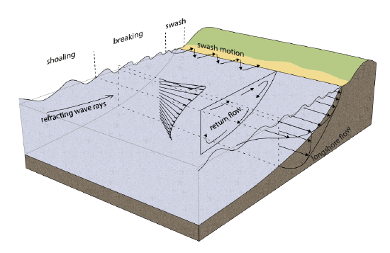
To this point, we have considered the undertow and alongshore current in isolation. In reality, the wave-induced current had a 3D structure, as can be seen in Fig. 5.44.


