5.6: Wind-induced set-up and currents

Moving air exerts a shear stress \(\tau\) on the water surface that can be modelled by, again, a quadratic friction law:

\[\tau_{\text{wind}} = C_d \rho_a W^2\]

where:

\(C_d\)	drag coefficient depending on wind velocity: \(C_d = (0.63 + 0.066 W) \times 10^{-3}\) for \(2 < W < 21m/s\) (Smith & Banke, 1975)
\(\rho_a\)	density of air (1.25 \(kg/m^3\))
\(W\)	wind velocity at the water surface

Due to this wind shear stress, the upper parts of the water layers will start to move more or less in the same direction as the wind direction. When the wind is seaward directed, a seaward directed current is generated in the upper water layers, the velocity of which is determined by the duration of the particular wind condition and its force.

Figure 5.50: Wind set-up balancing wind shear stress in the case of onshore wind on a shelf. In the deep ocean, the water set into motion in the upper layers can easily spread out. Vertical exchange of water makes this possible. On the shelf there is no escape due to limited water depth and the surface water is driven ashore.

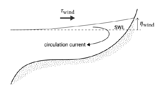
Similarly, a landward directed wind will induce a landward current in the upper layers. However, a coastline forms a barrier for this landward current and in an equilibrium situation the mean onshore directed flow should be zero (just as with the wave-induced flow). Therefore, to compensate for the landward (or seaward) directed water mass movement in the upper layers, an opposite directed water mass transport follows in the lower water layers. In addition to these ‘compensation currents’, a water level set-up or set-down develops near the coast to balance the wind-induced shear stresses (see Fig. 5.50)

The equilibrium condition is given by:

\[\rho g h \dfrac{d\bar{\eta}}{dx} = \tau_{\text{wind},x}\label{eq5.6.2}\]

Equation \(\ref{eq5.6.2}\) shows that the wind set-up is inversely proportional to the water depth. Hence, in the shallow coastal zone (up to the shelf break) water can pile up to great heights (storm surge).

When the wind is directed parallel to a (long) coast, a longshore current is generated. It takes some time (order of magnitude one day) for the wind-driven current to develop completely. In the equilibrium situation and in the absence of other driving forces, the wind shear stress and the bed shear stress are equal as was the case for the wave-induced longshore current.

Figure 5.51: Typical velocity distribution for wind-driven current.

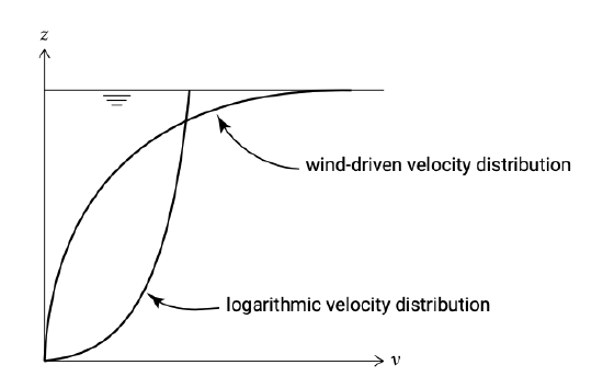
The vertical distribution of the wind-generated current differs substantially from the current generated by a water level gradient (Fig. 5.51). The highest flow velocities occur at the water surface, with usually a rapid decrease in the downward direction (much more than with the logarithmic velocity profile).

During storms, the wind stress may have an important effect on the residual longshore current. Often, however, the effect of wind stress on the longshore current in the littoral zone can be neglected. Besides, the morphological impact is limited due to the relatively small velocities near the bottom where the highest sediment concentrations occur.

Wind-driven currents are of greater importance in, for instance, coastal lagoons. The Dutch Wadden Sea is an example of a series of tidal basins in which wind-driven currents may play an important role. For dominant SW winds, a significant volume of water and sediment can be transported towards the east. This may lead to a gradual, but over the years continuing, shift of the watersheds between the barrier islands and the mainland. FitzGerald and Penland (1987) hypothesise that this primarily wind-generated transport is the main force behind inlet migration in the German Wadden Sea.

In Sect. 1.4.6, the phenomenon of storm surge was introduced. A storm surge is like a raised dome of water due to the combination of strong onshore winds (the above described wind set-up) and the lowered atmospheric pressure in a storm centre. The lower atmospheric pressure raises the water level. The coastal topography of the North Sea (shallow and funnel-shaped) and its predominantly westerly winds make it very susceptible to storm surges. The severity of a storm surge depends on its timing relative to the tidal cycle and the duration of the storm system. A storm system with a long duration (a few days) coinciding with spring tide can result in severe flooding of coastal areas. The storm surge height in the southern North Sea resulting in the 1953 flood event was 2.9 m and the storm duration was more than two days. Bangladesh experienced storm surge heights of around 9 m in 1970. Due to the lack of appropriate coastal protection this surge resulted in a very large number of casualties (500 000). Storm surges in the Bay of Bengal build up from tropical cyclones.