
5.7.2: Tidal propagation along the shore
- Page ID
- 16336

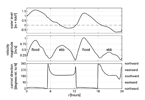
Figure 5.53 shows measured water level (vertical tide), current velocity (horizontal tide) and current directions for a location a few kilometres off the Dutch coast.
The flood-tidal current runs in the northward direction along the Dutch coast and the ebb current runs southward, in accordance with the direction of the rotary wave in ocean basins and seas in the Northern Hemisphere (Sect. 3.2). The flood and ebb velocities are maximum around high and low water respectively. The latter is characteristic of the propagation of the tide in relatively deep water, where bed friction has relatively little effect on the propagation. As explained in Sect. 3.8, under those circumstances, the tidal wave has a progressive character and water level and velocity are in phase (just as for wind waves). Figure 5.53 further shows that the tidal record deviates from an ideal symmetrical oscillation, which will be discussed later on in this section.
The effect of bottom friction
As previously, an alongshore uniform coast is considered with the \(y\)-axis defined parallel to the shoreline and the \(x\)-axis perpendicular to the shoreline. If the tidal elevation at lowest order is equal to \(\eta (t) = a \cos (\omega t - ky)\) the alongshore tidal velocity can be written as \(v(t) = V \cos (\omega t - ky - \varphi)\). For the M2 tide \(\omega \approx 1.4 \times 10^{-4} s^{-1}\).
For the Kelvin wave we found \(\varphi = 0\) for the propagation alongshore (Sect. 3.8). With the flood velocity defined as positive, \(\varphi = 0\) means that velocity and elevation are in phase (progressive wave). The Kelvin wave was found by solving the momentum balance in the \(x\)- and \(y\)-directions, Eqs. 3.8.3.4 and 3.8.3.5 and , and the continuity equation Eq. 3.8.3.6. We assumed that friction was very small compared to inertia.
In coastal engineering applications we generally consider the tidal flow in a zone relatively close to the coast (order 10 km). In that case we cannot neglect friction. If we neglect the inertia term \(\partial v/\partial t\) in Eq. 3.8.3.5, but add a friction term, the momentum equation (in the alongshore \(y\)-direction) becomes:
\[\xcancel{\underbrace{\dfrac{\partial v}{\partial t}}_{\text{inertia (local accelerations)}}} = \underbrace{-g \dfrac{\partial \eta}{\partial y}}_{\text{alongshore water level gradient}} \underbrace{-\dfrac{\tau_{by}}{\rho h}}_{\text{friction}}\label{eq5.7.2.1}\]
In this equation the alongshore pressure gradient \(\partial \eta /\partial y\) is constant in the cross-shore direction (for the narrow coastal strip under consideration). Although a quadratic friction law is more appropriate, for simplicity we assume that the friction is linearly dependent on the alongshore tidal velocity: \(\tau_{by} = \rho c_f v|v| \approx \rho rv\). Eq. \(\ref{eq5.7.2.1}\) now reads:
\[g \dfrac{\partial \eta}{\partial y} = -\dfrac{r}{h} v\label{eq5.7.2.2}\]
This equation suggests that the local nearshore water level gradient in a certain tidal phase is balanced by (linear) bed friction. Hence, the tidal velocity is not in phase with the tidal elevation but with the negative alongshore water level gradient. Or, to put it simply: at any point in time the water flows from a location with high water to a location with low water (not different from river flow, with the difference that the tide reverses direction). In this example the phase difference \(\varphi = -\pi /2\).
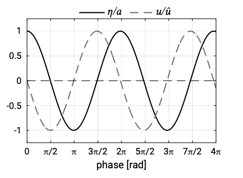
Figure 5.54 shows that for \(\varphi = -\pi /2 = -90^{\circ}\) the velocity leads the elevation by a quarter period or about 3 hours for the M2 tide. Figure 5.54 shows also that for the special case of \(\varphi = -\pi /2\):
- during the entire time it takes for the water to reach the lowest elevation (the falling period) the velocities are negative (ebb current);
- during the time it takes to reach the highest elevation (the rising period) the velocities are positive (flood current).
Thus: in the case that the velocity leads the surface elevation by 90°, the falling period coincides with the ebb duration and the rising period with the flood duration.
In general, the phase relationship between vertical and horizontal tide is very complex. Not only friction but also (partial) reflections of the tidal wave introduce phase differences between velocity and elevation. Generally, the phase difference \(\varphi\) in coastal waters and basins varies between zero and \(\varphi = -\pi /2\). If there is a phase difference between velocity and tidal elevation, it will be such that the velocity peaks before the tidal elevation.
The effect of friction is not only to introduce a phase difference between elevation and velocity, but to reduce their magnitudes as well compared to the same frictionless wave. In Sect. 5.7.3, the effects of friction and reflection are examined in more detail for the propagation into tidal basins.
Alongshore differences
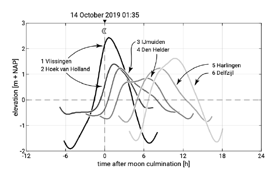
Along the Dutch coast the tidal wave propagates northwards. We saw that at lowest order the tidal elevation and velocity along the coast (\(y\)-direction) can be described by \(\eta = a \cos (\omega t - ky)\) and \(v = V \cos (\omega t - ky - \varphi)\). This means that the phase \(ky\) of the tide increases (or in other words: the wave form is delayed) from the delta area in the south towards the Wadden area in the north. This can be seen from Fig. 5.55.
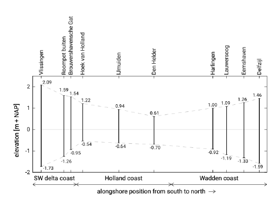
The figure shows that not only the phase \(ky\) differs along the coast, but the shapes and amplitudes as well. Figure 5.56 clearly shows that the tidal range is largest at Vlissingen (on average 3.8 m) and smallest around Den Helder (on average 1.3 m). Along the central Holland coast the average tidal range is \(2m\) at most7. Nevertheless, this tidal range is significantly larger than the tidal range from equilibrium theory. The along-shore differences are related to the position of the amphidromic points in the North Sea (see Fig. 3.31).
As opposed to the stochastic wind waves, the tidal motion is deterministic, viz. independent of weather or climatic conditions. Once the tidal constituents (amplitudes and phases) are known at certain measurement locations, the tide can be forecasted. Using a model based on momentum and continuity equations and data from measurements made simultaneously at different points along the coast, the tide at locations different from the measurement locations can be forecasted as well.
Skewness and asymmetry
Figures 5.55 and 5.56 indicate that the tidal curves deviate from an ideal symmetrical tide. We see that:
- high water is further above the mean than low water is below it; this also implies a shorter duration of positive water levels than negative water levels; this type of asymmetry is equivalent to the skewed wind waves in the shoaling zone with long, flat troughs and narrow, peaked crests (see Sect. 5.3). In Vlissingen the skewness of the tidal elevation is positive and in Den Helder negative.
- the time it takes for the water to reach the lowest elevation (the falling period) is not equal to the time it takes to reach the highest elevation (the rising period). The resulting shape of the tidal curve is asymmetric about the vertical axis, comparable with the asymmetry in wind waves just before breaking.
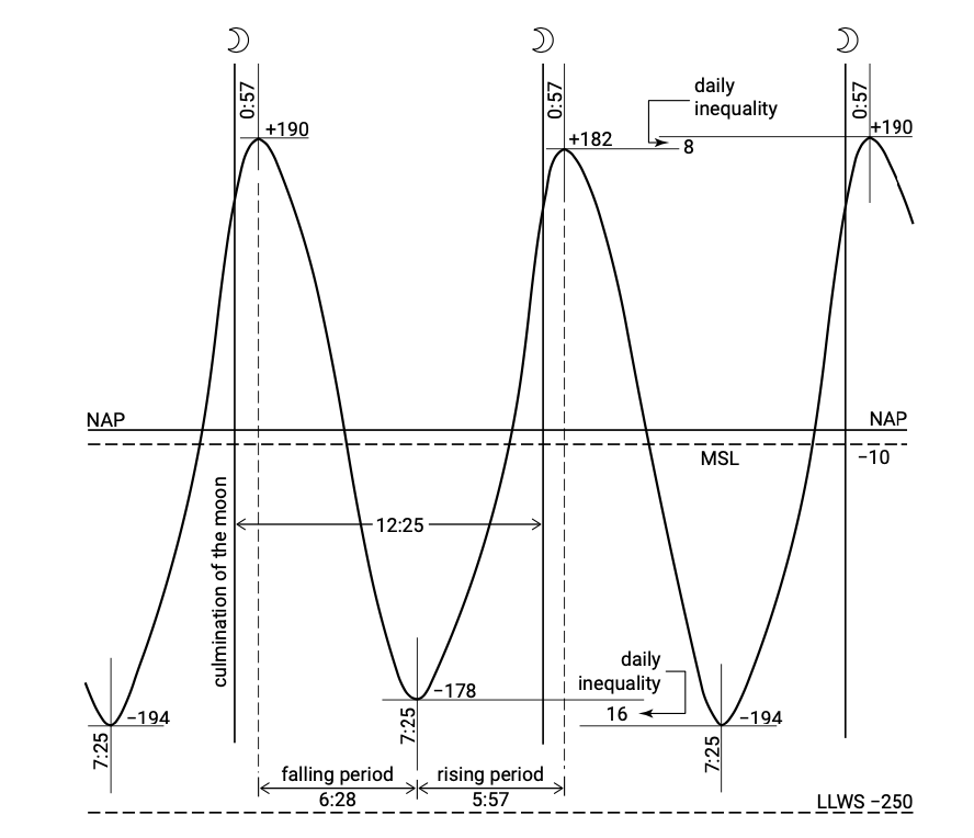
Figure 5.57 shows in more detail the average tidal curve for Vlissingen. It shows a falling period of \(6.28\ h\) and a rising period of \(5.57\ h\). Although the exact ratios vary, for all stations along the Dutch coast the falling period is longer than the rising period. For instance in IJmuiden the falling period and rising period are \(8.03\ h\) and \(4.22\ h\) respectively. This phenomenon is often referred to as tidal asymmetry.
The longer falling period can be explained from the phase velocity for shallow water \(c = \sqrt{g(h + \eta )}\). For high tide (\(\eta\) positive) the propagation velocity is larger than for low tide (\(\eta\) negative). Since the high tide (the wave crest) propagates faster than the low tide (the trough), the rising period is smaller than the falling period. This generally holds for the open coast, but in basins this may be different.
When it is said that the (vertical) tide is flood-dominant this refers to a shorter rising period than falling period. Vice versa ebb-dominance indicates a shorter falling period. For the reasons mentioned in Sect. 5.7.1 these terms flood- and ebb-dominance in relation to the vertical tide may be confusing. We will therefore use flood (or ebb) dominance only to indicate the direction of net sediment transport (see Sect. 9.7) as a result of asymmetries of the horizontal tide.
Like the vertical tide, the horizontal tide may display both skewness and asymmetry:
- the average peak flood current may be stronger than the average peak ebb current, which leads to a shorter flood duration than ebb duration (or vice versa);
- the velocity signal may be asymmetric around the vertical, which means that the rate at which the velocity changes around slack water (= flow reversal) is different when changing from ebb to flood than when changing from flood to ebb (see for instance Fig. 5.52).
Figure 5.53 shows that if the horizontal and vertical tide are in phase, the skewed and asymmetric tidal elevation directly translates in similar characteristics for the tidal velocity. In basins the relationship between the vertical and horizontal tide can be more complex. Tidal asymmetry will be discussed in more detail in Sect. 5.7.4.
Cross-shore distribution of the tidal velocity
Surface waves refract towards the coast and generate a longshore current along the coast. Tidal propagation tends to be along a coast or channel. Hence, both wave-induced longshore current and tidal currents are mainly parallel to the coast (see Fig. 5.58). The direction of the tidal current reverses during the tidal cycle. Alongshore tidal velocities in shallow water can be anything from a few decimetres per second to several metres per second.
In very shallow water the inertia effect is small and the velocity at any moment in the tide is governed by the balance between alongshore water level gradient and friction.
According to Eq. \(\ref{eq5.7.2.2}\), the velocity magnitude is at every moment of the tidal phase linearly dependent on the water depth and the alongshore water level gradient. If we use a quadratic friction law with a constant friction factor, the velocity magnitude is proportional to the square root of the product of water depth and alongshore water level gradient:
\[v \propto \sqrt{h \dfrac{\partial \eta}{\partial y}}\label{eq5.7.2.3}\]
If the tidal velocity at one particular water depth is known, for instance from measurements, then a very practical method for finding the cross-shore distribution of the velocities is by using Eq. \(\ref{eq5.7.2.3}\). This leads to:
\[v_2 = v_1 \sqrt{\dfrac{h_2}{h_1}}\]
where:
| \(v_{1,2}\) | tidal current velocities at cross-shore positions 1 and 2 | \(m/s\) |
| \(h_{1,2}\) | still water depth at points 1 and 2 | \(m\) |
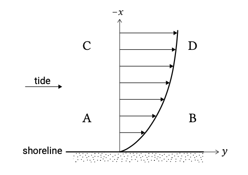
Note that in this approach it is assumed that the alongshore water level gradient does not vary in the cross-shore direction (head between D and C in Fig. 5.58 is equal to head between B and A). Following this simple approach, a tidal alongshore velocity of \(0.7\ m/s\) at a water depth of 10 m yields a tidal velocity of \(0.3\ m/s\) at a water depth of only \(2\ m\). In this shallow region with \(2\ m\) water depth, waves can be very effective in increasing the bed shear stress (the wave boundary layer acts as an extra resistance for the flow). Consequently, the tidal velocities in the wave-influenced littoral zone will even be smaller.
Effect of tide on wave-generated longshore current
The tide influences the wave-generated longshore current in the breaker zone. One complicating factor here is that the direction of the tidal velocity changes twice during one tidal cycle. The appropriate way to include the effect of tides is first to combine the driving forces (during ebb and flood periods) and then to calculate the velocity. Simply adding the tidal velocity to the wave-induced longshore current is not correct (that would only be possible if the velocity is a linear function of the driving force, which is not the case).
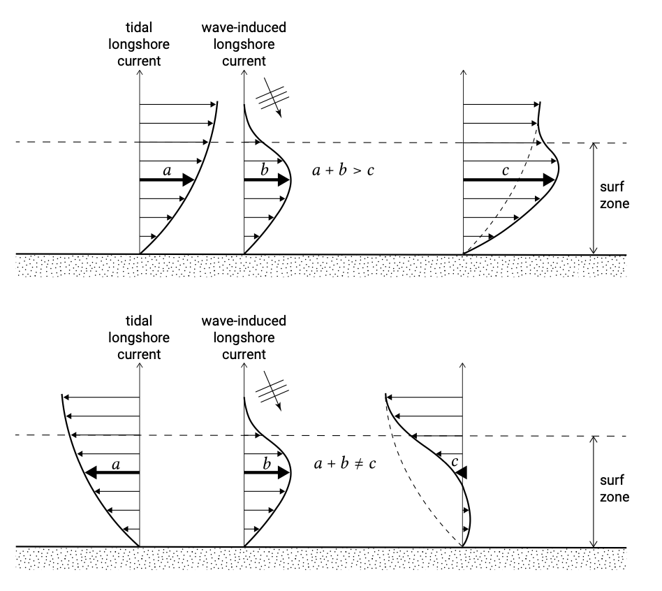
Figure 5.59 shows the velocity distribution for the combination of wave-generated currents with ebb and flood tidal velocities. The maximum tidal velocity occurs outside the breaker zone, but the effect inside the breaker zone can be quite substantial. If the tidal force is in the same direction as the wave-driven current, the maximum along-shore flow velocity increases (and shifts towards the breaker line). If the tidal force is in the opposite direction, the maximum velocity decreases (and shifts towards the shoreline). The longshore current in the breaker zone, although reduced in velocity, might then be in the opposite direction as the tidal current present further seawards.
If the wave-induced alongshore driving forces are large enough relative to the tidal forces, the tidal current in the breaker zone may be overshadowed by the wave-induced longshore current. Flow reversal with the tide may not occur.
Tidal currents may significantly complicate the determination of the longshore current in the breaker zone. In practical cases, like for instance for the Dutch coast, it will be necessary to establish the longshore current throughout the entire tidal cycle. Only in areas with weak tidal forces (like for instance the Mediterranean) the effect of tides on the water movement in the breaker zone can be neglected.
Tidal currents around structures
Structures tend to divert the tidal flow especially when they extend far seaward. The harbour moles of IJmuiden, the sea port of Amsterdam, were extended to approximately 2500 m in the period of 1962 to 1968. The convergence of the tidal flow (contraction of the streamlines) around this breakwater led to relatively high velocities in front of the harbour entrance, where subsequently a scour hole developed. Another example is the long dam that has been constructed at the Dutch Wadden Sea island of Texel in 1995.
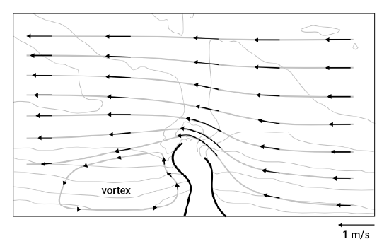
Figure 5.60 schematically shows the deflection of tidal currents by IJmuiden harbour. Due to the tidal variation the flow field is not stationary. The depicted flow field represents the ebb flow. Near the harbour entrance a flow contraction can be noticed, while downstream from the harbour moles an eddy is visible. A simple rule of thumb states that the alongshore length of the eddy should be – in a stationary situation – around six times the length of the harbour mole. Due to the tide reversal however, the growth of the eddy is restricted. The flow patterns have implications for the sediment transport and resulting morphology.
In this study the harbour basin itself was not included in the computation. The tidal flow passing the harbour entrance can drive an eddy in the harbour basin. This can lead to an exchange of water and sediment between the harbour and the area outside.
7. The spring tidal range however is everywhere at least \(2m\). Therefore, the Dutch coast qualifies as a meso-tidal regime, see Sect. 4.4.1.