5.5.4: Cross-shore balance-wave set-up and set-down

Wave forces have an effect on the mean flow; they induce mean water level variations (set-down, set-up) and mean currents (a longshore current in the case of waves obliquely approaching the shore).

First we consider the wave force in the cross-shore direction (given by Eq. 5.5.3.1). For illustration purposes we consider the simplified situation of a long-crested wave normally incident to straight and parallel depth contours (parallel to the \(y\)-axis, \(\theta = \varphi = 0\)). This means that there are no gradients in the alongshore direction: the situation is alongshore uniform (all \(y\)-derivatives are zero) and the wave force reduces to Eq. 5.5.3.2.

Cross-shore mass balance (alongshore uniform coast)

In a stationary case the cross-shore current averaged over the entire water column must be zero (since water neither piles up higher and higher against the coast nor flows towards deeper water). At every point in the cross-shore profile, the onshore directed mass-flux near the water surface is therefore compensated by an offshore directed return current at lower elevations, such that the net depth-averaged flow through each cross-section is zero (see Fig. 5.25). The offshore directed depth-mean velocity under the wave trough level can be found from Eq. 5.5.1.4.

Cross-shore momentum balance (alongshore uniform coast)

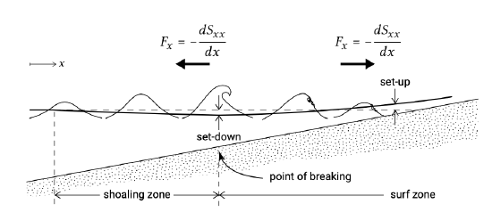
Figure 5.32: In the shoaling zone, \(S_{xx}\) increases in landward direction resulting in a wave force acting in seaward direction and a lowering of the mean water level towards the breaking point. Wave breaking in the surf causes \(S_{xx}\) to decrease in landward direction, such that an onshore wave forces raises the water level towards the shore (set-up).

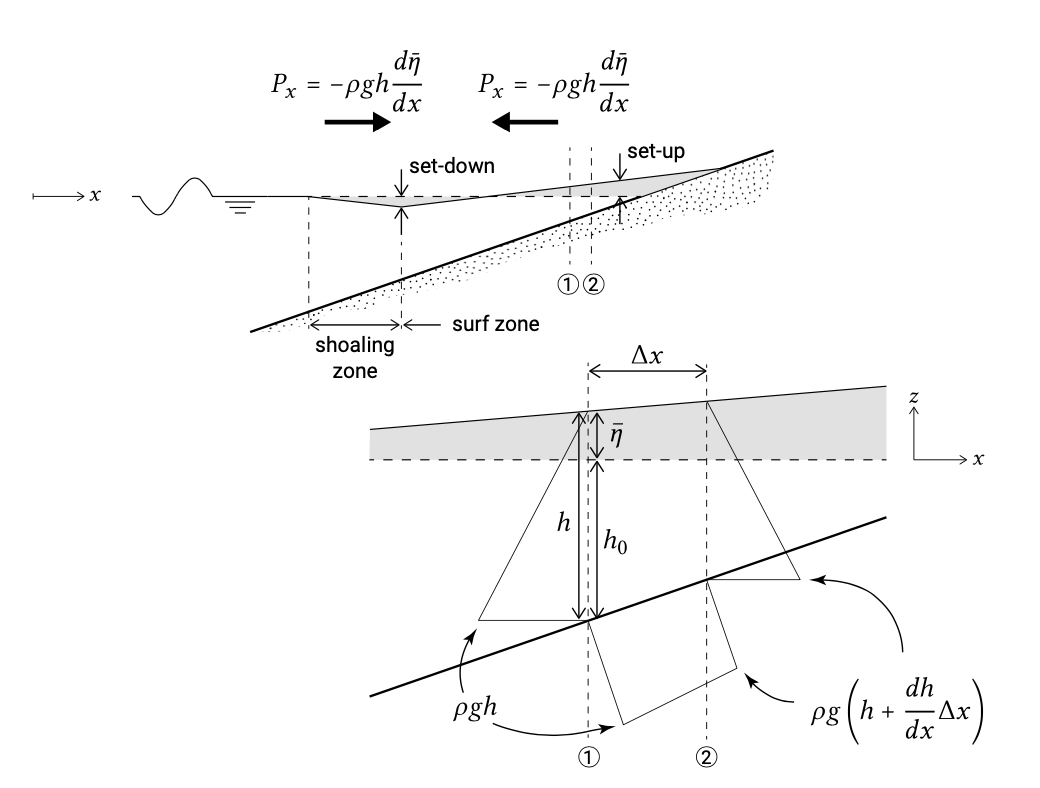
Figure 5.33: The control volume for a simple cross-shore momentum balance between two locations 1 and 2. The radiation stress is \(S_{xx,1}\) at location 1 and \(S_{xx, 2}\) at location 2. The triangles and quadrangle indicate the pressure forces. If locations 1 and 2 are in the surf zone, the onshore directed wave force (onshore since \(S_{xx, 1} > S_{xx, 2}\)) is balanced by a net offshore pressure force (through a raising of the water level towards the coast).

The wave force is determined by the cross-shore gradient of \(S_{xx}\). The magnitude of the radiation stress \(S_{xx} = (2n - 1/2) E\) in the wave propagation direction depends on the wave height, the water depth and the wavelength. Based on energy conservation Sect. 5.2.2 showed that the wave energy (wave heights) tends to increase when the waves approach the surf zone (after a small initial decrease). Since \(n\) increases in intermediate water depths, \(S_{xx}\) increases in the shoaling region. Further offshore in really deep water, the radiation stress \(S_{xx}\) is constant. An increasing \(S_{xx}\) in the landward direction means that at a water column a resulting force due to radiation stresses is acting in the seaward direction (see Figs. 5.31 and 5.32). A (small) difference in water level at both sides of the water column (lower towards the coast) ensures that equilibrium of forces is achieved again. This phenomenon is called wave set-down, which means that outside the breaker zone in intermediate water depths, the water level at the landward side of a water column is a bit lower than at the seaward side (see Figs. 5.32 and 5.33, top figure). Inside the surf zone the magnitude of \(S_{xx}\) decreases rapidly due to wave breaking while moving towards the waterline. The decrease in \(S_{xx}\) is equivalent to a force in the landward direction (see Fig. 5.32). To achieve equilibrium again, the water level at the landward side of the column should be higher than at the seaward side (wave set-up, see Fig. 5.32) creating a seaward directed pressure force (see Fig. 5.33, upper plot).

The lower figure of Fig. 5.33 illustrates the cross-shore balance of momentum between two (arbitrary) points 1 and 2. The net pressure force (per unit alongshore distance) is \(P_x \Delta x = -\rho g h d \bar{\eta}/dx \Delta x\). It consists of:

• the hydrostatic force \(1/2 \rho g h^2\) at point 1; minus
• the hydrostatic force \(1/2 \rho g (h + dh/dx \Delta x)^2 \approx 1/2 \rho g h^2 + \rho g h dh/dx \Delta x\) at point 2; minus
• the horizontal component \(\approx \rho g h (dh_0/dx \Delta x)\) of the hydrostatic force along the bottom.

Figure 5.34: The force balance between wave force and pressure force reads \(F_x + P_x = 0\). In the surf zone \(F_x\) is positive (landward directed) and \(P_x\) is negative (seaward directed).

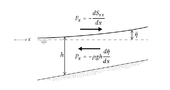
The equilibrium between the radiation stress gradient and pressure term due to the water level slope (see Fig. 5.34) yields the following first order differential equation:

\[F_x = -\dfrac{dS_{xx}}{dx} = \rho g h \dfrac{d\bar{\eta}}{dx} = \rho g (h_0 + \bar{\eta}) \dfrac{d\bar{\eta}}{dx}\label{eq5.5.4.1}\]

where:

\(x\)	co-ordinate axis pointing from land to sea	\(m\)
\(h_0\)	still-water depth at point \(x\) (in absence of waves)	\(m\)
\(\bar{\eta}\)	wave-induced water level set-up at point \(x\)	\(m\)

Eq. \(\ref{eq5.5.4.1}\) is the depth-integrated cross-shore momentum equation for a stationary along-shore uniform situation. This balance in the cross-shore direction holds both for obliquely and normally incident waves. We have not included bottom friction in this equation, because it is generally assumed to be an order of magnitude smaller than the other terms in the equation⁶. Also the Coriolis term is assumed to be small compared to the wave forcing. The equation is valid inside and outside the surf zone under the conditions listed above.

Note that inside (outside) the surf zone the term \(dS_{xx}/dx\) is negative (positive) yielding a positive (negative) water level gradient (\(d\bar{\eta}/dx\)), see Figs. 5.32 and 5.34.Therefore, the still water surface becomes lower in the shoaling region (set-down). Moving inside the surf zone towards the waterline, the still water surface becomes higher (set-up). In order to calculate the wave set-up (and set-down) we need to assess the radiation stress terms inside and outside the surf zone and integrate Eq. \(\ref{eq5.5.4.1}\) with respect to \(x\).

With Eq. 5.5.2.11 we can write Eq. \(\ref{eq5.5.4.1}\) as:

\[-\dfrac{d}{dx} \left [\left (n - \dfrac{1}{2} + n \cos^2 \theta \right ) E \right ] = \rho g h \dfrac{d\bar{\eta}}{dx}\label{eq5.5.4.2}\]

The spatial wave energy variation must be solved from conservation of energy, Eq. 5.2.1.2, which reduces to \(d(Ec_g \cos \theta )/dx = -D_w\) under the present assumptions.

Simple model for wave set-down in the case of normally incident waves

For waves normally incident to an alongshore uniform coast (\(\theta = \varphi = 0\)) and under the assumption of shallow water (\(n = 1\)) the momentum balance Eq. \(\ref{eq5.5.4.2}\) can be written as:

\[-\dfrac{d}{dx} \left (\dfrac{3}{2} E\right ) = \rho g h \dfrac{d\bar{\eta}}{dx}\label{eq5.5.4.3}\]

Section 5.2.2 gave us the following energy balance for a normally incident shoaling wave:

\[\dfrac{H_2}{H_1} = \sqrt{\dfrac{c_{g.1}}{c_{g,2}}}\label{eq5.5.4.4}\]

Amongst others Longuet-Higgins and Stewart (1962) derived an expression for the set-down for regular waves by integration of Eq. \(\ref{eq5.5.4.3}\) using the energy balance of shoaling waves Eq. \(\ref{eq5.5.4.4}\). The integration constant is determined from \(\bar{\eta} = 0\) in deep water. It can be shown that in the shallow water approximation the set-down then equals:

\[\bar{\eta} = -\dfrac{1}{16} \dfrac{H^2}{h}\]

For waves propagating without dissipation towards the shore, the wave height increases and the water depth decreases. Hence, the set-down gradually increases in magnitude to a maximum just outside the breaker zone at the point where the waves start breaking. At the breaker point the set-down equals:

\[\overline{\eta_b} = -\dfrac{1}{16} \dfrac{H_b^2}{h_b} = -\dfrac{1}{16} \gamma H_b\]

where:

\(\overline{\eta_b}\)	water level change at the point of wave breaking	\(m\)
\(\gamma\)	wave breaking index (\(H_b/h_b\))	-
\(H_b\)	wave height at point of breaking	\(m\)
\(h_b\)	still water depth at point of breaking	\(m\)

Thus, with \(\gamma\) put equal to 0.8 the set-down at the point of breaking is 4% of the local water depth.

Analytical model for set-up in the case of normally incident waves

Figure 5.35: Set-down and set-up and equilibrium of forces in the entire breaker zone.

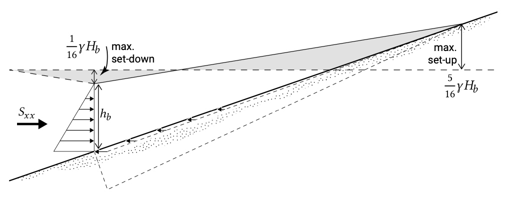
Inside the surf zone model the dissipation due to wave breaking needs to be included in the energy balance. In the following an analytical expression for wave set-up is derived using a very simple dissipation model and assuming normally incident waves. The derivation considers equilibrium of forces for the entire breaker of surf zone (see Fig. 5.35).

A simple model for the energy dissipation due to wave breaking assumes that the wave height everywhere in the surf zone is proportional to the local water depth: everywhere in the surf zone \(H = \gamma h\) (see Eq. 5.2.5.4). If we further use the shallow water approximation (\(n = 1\)), then it follows that \(S_{xx} = 3/2 E\) is decreasing from the breaker line towards the coastline. Following similar reasoning to the previous section, this causes landward directed resulting forces acting on a water column. This will be balanced by a water level increase (in the landward direction) over the water column. If we substitute \(S_{xx} = 3/2 E = 3/16 \rho g H^2 = 3/16 \rho g \gamma^2 h^2\) in Eq. \(\ref{eq5.5.4.3}\) we find the following balance:

\[-\dfrac{d}{dx} [3/16 \gamma^2 h^2] = h \dfrac{d\bar{\eta}}{dx}\]

and thus:

\[\dfrac{d\bar{\eta}}{dx} = -3/8 \gamma^2 \dfrac{dh}{dx} \label{eq5.5.4.8}\]

Substituting \(h = h_0 + \bar{\eta}\) in Eq. \(\ref{eq5.5.4.8}\) gives:

\[\dfrac{d \bar{\eta}}{dx} = -\dfrac{3/8 \gamma^2}{(1 + 3/8 \gamma^2)} \dfrac{dh_0}{dx}\label{eq5.5.4.9}\]

Hence, because the water depth decreases in the surf zone (\(dh_0/dx < 0\)), the setup increases (\(d\bar{\eta}/dx >0\)). With a constant bottom slope and a constant breaker index, the water level slope inside the breaker zone is constant.

Equation \(\ref{eq5.5.4.8}\) – or equivalently Eq. \(\ref{eq5.5.4.9}\), which gives a bit more involved math – can be integrated from the breaker point to the water line to get the wave set-up throughout the surf zone (using \(\bar{\eta} = \bar{\eta}_b\) for \(h = h_b\) to find the integration constant \(C\)):

\[\bar{\eta} = -\dfrac{3}{8} \gamma^2 h + C = \bar{\eta}_b + 3/8 \gamma^2 (h_b - h)\]

At the shoreline the water depth \(h\) is zero and we find for the set-up at the water line:

\[\bar{\eta}_{\text{shore}} = \bar{\eta}_{b} + 3/8 \gamma^2 h_b = \bar{\eta}_b + 3/8 \gamma H_b\]

The water level \(\Delta \bar{\eta}\) difference between the breaker line and the point of maximum water level rise (wave set-up) equals:

\[\Delta \bar{\eta} = \dfrac{3}{8} \gamma H_b\]

With \(\gamma = 0.8\) this amounts to \(0.3 H_b\). Wave set-up can thus be quite significant, as is further illustrated in Example 5.5.4.1. Since the maximum set-down at the breaker line is \(1/16 \gamma H_b\), the maximum wave set-up relative to the still water level is \(5/16 \gamma H_b\) (see Fig. 5.35).

Exercise \(\PageIndex{1}\)

Input parameters

Offshore wave height \(H_0 = 5 m\)
Wave period \(T = 12 s\)
Offshore wave direction \(\varphi_0 = 0^{\circ}\) (normally incident)
Breaker index \(\gamma = 0.7\)

Required Maximum wave set-up relative to the still water level

Output The first step is to compute the wave height at the breaker line. \(H_b\) depends on shoaling and (though not in this case) refraction. Computer programs can be used or linear wave theory using the following iterative steps (for an arbitrary wave angle):

1. Guess a breaker depth, \(h_b\) and compute \(h_b/L_0\)
2. Using Table A.3 in App. A to determine the shoaling coefficient \(K_{sh}\) and the ratio of wave speeds \(c/c_0\)
3. Determine the angle \(\varphi\) using \(\sin \varphi = c/c_0 \sin \varphi_0\)
4. Compute the wave height at water depth \(h_b\) from \(H = H_0 K_{sh} (\cos \varphi_0 /\cos \varphi)\)
5. Check whether \(H/h_b = \gamma = 0.7\). If yes: o.k.; if no: return to step 1 with a better guess of \(h_b\)

In this case of normally incident waves, step 3 can be omitted. It follows that \(H_b = 5.5 m\). The maximum wave set-up then becomes \(5/16 \gamma H_b = 1.2 m\) above still water level.

Conclusion If we assume an average beach slope of 1:50, then almost 60 m of beach width is ‘lost’ by the effect of wave set-up.

Summary

• In the shoaling zone \(S_{xx}\) increases in the positive \(x\)-direction (the cross-shore direction); the positive gradient in \(S_{xx} (\partial S_{xx}/\partial x > 0)\) is equivalent to a force \(F_x\) directed in the offshore direction. This is compensated for by an onshore directed pressure force due to a set-down (lowering of the water level). The set-down can be approximated as \(1/16 \gamma H_b\);
• In the surf zone \(S_{xx}\) decreases in the positive \(x\)-direction; the resulting negative gradient in \(S_{xx} (\partial S_{xx}/\partial x < 0)\) is equivalent to a force \(F_x\) directed in the onshore direction. This is balanced by an offshore directed pressure force due to wave set-up (raising of the water level towards the water line). The maximum wave set-up relative to the still water level is \(5/16 \gamma H_b\).

Concluding remarks

• The wave height increase in the shoaling zone as well as the wave height decay in the surf zone can be predicted reasonably well using a wave action or energy balance. When assuming (as we did) that inside the surf zone there is a direct relationship between the local wave height and local water depth, the build up of the wave set-up starts at the (first) point of breaking. In reality there is a delay in the transfer of momentum from the wave motion to the mean flow. This means that the set-up (and also the start of the build up of the longshore current) is shifted in the landward direction. The delay may be caused by the temporary storage of energy and momentum in surface rollers of breaking waves. In this way the dissipation process is delayed, hence shifting the region of wave set-up in the shoreward direction. This temporary storage can be modelled using a roller model and a roller energy balance;
• Waves are irregular. For the computation of the wave set-up for irregular waves, the root mean square wave height \(H_{rms}\) is generally applied;
• In an irregular wave field, wave heights vary on the wave group scale (Sect.5.8.2). That means that the magnitude of the radiation stress varies on the wave group scale as well. This time-varying force generates water level fluctuations with a timescale much longer than the wave period (long waves);
• Waves generally approach the coastline under a (small) angle that decreases in smaller water depths. Therefore \(S_{xx}\), the cross-shore gradients of \(S_{xx}\) and the set-up are smaller than for normally incident waves.

---

6. Apotsos et al. (2007) showed that this assumption may result in underprediction of the set-up. For simplicity however, bottom stress is often neglected, also in these lecture notes.