
11: Appendix A - Linear wave theory
- Page ID
- 16455

\( \newcommand{\vecs}[1]{\overset { \scriptstyle \rightharpoonup} {\mathbf{#1}} } \)
\( \newcommand{\vecd}[1]{\overset{-\!-\!\rightharpoonup}{\vphantom{a}\smash {#1}}} \)
\( \newcommand{\dsum}{\displaystyle\sum\limits} \)
\( \newcommand{\dint}{\displaystyle\int\limits} \)
\( \newcommand{\dlim}{\displaystyle\lim\limits} \)
\( \newcommand{\id}{\mathrm{id}}\) \( \newcommand{\Span}{\mathrm{span}}\)
( \newcommand{\kernel}{\mathrm{null}\,}\) \( \newcommand{\range}{\mathrm{range}\,}\)
\( \newcommand{\RealPart}{\mathrm{Re}}\) \( \newcommand{\ImaginaryPart}{\mathrm{Im}}\)
\( \newcommand{\Argument}{\mathrm{Arg}}\) \( \newcommand{\norm}[1]{\| #1 \|}\)
\( \newcommand{\inner}[2]{\langle #1, #2 \rangle}\)
\( \newcommand{\Span}{\mathrm{span}}\)
\( \newcommand{\id}{\mathrm{id}}\)
\( \newcommand{\Span}{\mathrm{span}}\)
\( \newcommand{\kernel}{\mathrm{null}\,}\)
\( \newcommand{\range}{\mathrm{range}\,}\)
\( \newcommand{\RealPart}{\mathrm{Re}}\)
\( \newcommand{\ImaginaryPart}{\mathrm{Im}}\)
\( \newcommand{\Argument}{\mathrm{Arg}}\)
\( \newcommand{\norm}[1]{\| #1 \|}\)
\( \newcommand{\inner}[2]{\langle #1, #2 \rangle}\)
\( \newcommand{\Span}{\mathrm{span}}\) \( \newcommand{\AA}{\unicode[.8,0]{x212B}}\)
\( \newcommand{\vectorA}[1]{\vec{#1}} % arrow\)
\( \newcommand{\vectorAt}[1]{\vec{\text{#1}}} % arrow\)
\( \newcommand{\vectorB}[1]{\overset { \scriptstyle \rightharpoonup} {\mathbf{#1}} } \)
\( \newcommand{\vectorC}[1]{\textbf{#1}} \)
\( \newcommand{\vectorD}[1]{\overrightarrow{#1}} \)
\( \newcommand{\vectorDt}[1]{\overrightarrow{\text{#1}}} \)
\( \newcommand{\vectE}[1]{\overset{-\!-\!\rightharpoonup}{\vphantom{a}\smash{\mathbf {#1}}}} \)
\( \newcommand{\vecs}[1]{\overset { \scriptstyle \rightharpoonup} {\mathbf{#1}} } \)
\(\newcommand{\longvect}{\overrightarrow}\)
\( \newcommand{\vecd}[1]{\overset{-\!-\!\rightharpoonup}{\vphantom{a}\smash {#1}}} \)
\(\newcommand{\avec}{\mathbf a}\) \(\newcommand{\bvec}{\mathbf b}\) \(\newcommand{\cvec}{\mathbf c}\) \(\newcommand{\dvec}{\mathbf d}\) \(\newcommand{\dtil}{\widetilde{\mathbf d}}\) \(\newcommand{\evec}{\mathbf e}\) \(\newcommand{\fvec}{\mathbf f}\) \(\newcommand{\nvec}{\mathbf n}\) \(\newcommand{\pvec}{\mathbf p}\) \(\newcommand{\qvec}{\mathbf q}\) \(\newcommand{\svec}{\mathbf s}\) \(\newcommand{\tvec}{\mathbf t}\) \(\newcommand{\uvec}{\mathbf u}\) \(\newcommand{\vvec}{\mathbf v}\) \(\newcommand{\wvec}{\mathbf w}\) \(\newcommand{\xvec}{\mathbf x}\) \(\newcommand{\yvec}{\mathbf y}\) \(\newcommand{\zvec}{\mathbf z}\) \(\newcommand{\rvec}{\mathbf r}\) \(\newcommand{\mvec}{\mathbf m}\) \(\newcommand{\zerovec}{\mathbf 0}\) \(\newcommand{\onevec}{\mathbf 1}\) \(\newcommand{\real}{\mathbb R}\) \(\newcommand{\twovec}[2]{\left[\begin{array}{r}#1 \\ #2 \end{array}\right]}\) \(\newcommand{\ctwovec}[2]{\left[\begin{array}{c}#1 \\ #2 \end{array}\right]}\) \(\newcommand{\threevec}[3]{\left[\begin{array}{r}#1 \\ #2 \\ #3 \end{array}\right]}\) \(\newcommand{\cthreevec}[3]{\left[\begin{array}{c}#1 \\ #2 \\ #3 \end{array}\right]}\) \(\newcommand{\fourvec}[4]{\left[\begin{array}{r}#1 \\ #2 \\ #3 \\ #4 \end{array}\right]}\) \(\newcommand{\cfourvec}[4]{\left[\begin{array}{c}#1 \\ #2 \\ #3 \\ #4 \end{array}\right]}\) \(\newcommand{\fivevec}[5]{\left[\begin{array}{r}#1 \\ #2 \\ #3 \\ #4 \\ #5 \\ \end{array}\right]}\) \(\newcommand{\cfivevec}[5]{\left[\begin{array}{c}#1 \\ #2 \\ #3 \\ #4 \\ #5 \\ \end{array}\right]}\) \(\newcommand{\mattwo}[4]{\left[\begin{array}{rr}#1 \amp #2 \\ #3 \amp #4 \\ \end{array}\right]}\) \(\newcommand{\laspan}[1]{\text{Span}\{#1\}}\) \(\newcommand{\bcal}{\cal B}\) \(\newcommand{\ccal}{\cal C}\) \(\newcommand{\scal}{\cal S}\) \(\newcommand{\wcal}{\cal W}\) \(\newcommand{\ecal}{\cal E}\) \(\newcommand{\coords}[2]{\left\{#1\right\}_{#2}}\) \(\newcommand{\gray}[1]{\color{gray}{#1}}\) \(\newcommand{\lgray}[1]{\color{lightgray}{#1}}\) \(\newcommand{\rank}{\operatorname{rank}}\) \(\newcommand{\row}{\text{Row}}\) \(\newcommand{\col}{\text{Col}}\) \(\renewcommand{\row}{\text{Row}}\) \(\newcommand{\nul}{\text{Nul}}\) \(\newcommand{\var}{\text{Var}}\) \(\newcommand{\corr}{\text{corr}}\) \(\newcommand{\len}[1]{\left|#1\right|}\) \(\newcommand{\bbar}{\overline{\bvec}}\) \(\newcommand{\bhat}{\widehat{\bvec}}\) \(\newcommand{\bperp}{\bvec^\perp}\) \(\newcommand{\xhat}{\widehat{\xvec}}\) \(\newcommand{\vhat}{\widehat{\vvec}}\) \(\newcommand{\uhat}{\widehat{\uvec}}\) \(\newcommand{\what}{\widehat{\wvec}}\) \(\newcommand{\Sighat}{\widehat{\Sigma}}\) \(\newcommand{\lt}{<}\) \(\newcommand{\gt}{>}\) \(\newcommand{\amp}{&}\) \(\definecolor{fillinmathshade}{gray}{0.9}\)In the theory for linear waves, equations are given for properties like:
| the particle velocity \((u, w)\) at any height in the water column | \(m/s\) |
| the particle acceleration \((a_x, a_z)\) at any height in the water column | \(m^2/s\) |
| the particle displacement \((\xi , \zeta)\) at any height in the water column | \(m\) |
| the pressure (\(p\)) at any height in the water column | \(N/m^2\) |
| the wave speed (\(c\)) | \(m/s\) |
| the wave group speed \((c_g)\) | \(m/s\) |
| the wavelength \((L)\) | \(m\) |
| the wave profile (\(\eta\)) | \(m\) |
| the wave energy per wavelength per unit crest length \((E_t)\) | \(J/m\) |
| the energy per unit water surface area \((E)\) | \(J/m^2\) |
| the wave power \((U)\) | \(J/m \times s\) |
The general equations for these properties can be found in Table A.2 in the ‘Transitional Water Depth’ column. The equations for transitional water depth contain hyperbolic functions. It may be helpful to use standard tables containing the values of the hyperbolic functions. These tables can be found in the Coastal Engineering Manual. An extract of these tables is given in Table A.3.
Table A.1: Criteria for deep and shallow water waves with an error of the order of 1%
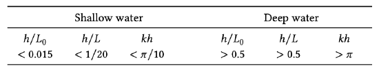
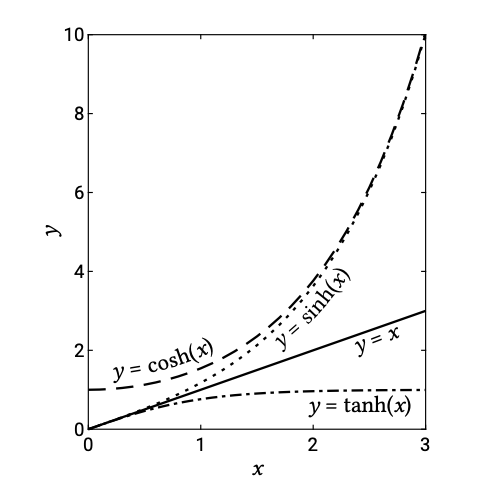
For the limiting cases of deep and shallow water (see Table A.1), simplifications can be made in the hyperbolic functions (see also Fig. A.1).
For relative deep water (\(h > L/2\) so \(kh > \pi\) where \(k = 2\pi /L\) is the wavenumber):
\[\sinh kh = \dfrac{1}{2} (e^{kh} - e^{-kh}) = \dfrac{1}{2} e^{kh} \ \ \ \ \ \ \text{ for } kh \to \infty\]
\[\cosh kh = \dfrac{1}{2} (e^{kh} + e^{-kh}) = \dfrac{1}{2} e^{kh} \ \ \ \ \ \ \text{ for } kh \to \infty\]
\[\tanh kh = 1 \ \ \ \ \ \ \ \ \ \ \ \ \ \ \ \ \ \ \ \ \ \ \ \ \ \ \ \ \ \ \ \ \ \ \ \ \ \ \ \text{ for } kh \to \infty\]
For relatively shallow water (\(h < L/20\) so \(kh < \pi /10\)):
\[\sinh kh = kh \ \ \ \ \ \ \ \text{ for } kh \to 0\]
\[\cosh kh = 1 \ \ \ \ \ \ \ \ \text{ for } kh \to 0\]
\[\tanh kh = kh \ \ \ \ \ \ \ \text{ for } kh \to 0\]
Table A.2: Expressions for shallow, transitional and deep water wave computations according to linear wave theory. Note that as opposed to the definitions in Chapters 3 and 5, \(z = 0\) at the the bottom (instead of \(z = -h\)) and \(z = h\) at the mean water level (instead of \(z = 0\)).
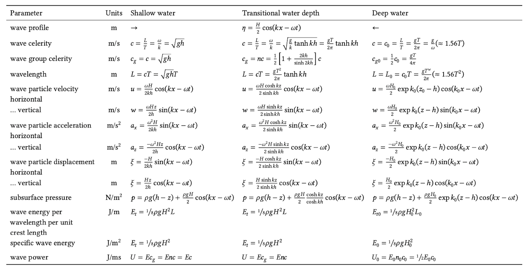
Of the equations in Table A.2 the following are frequently used in these lecture notes:
\[\omega^2 = \left ( \dfrac{2\pi }{T} \right )^2 = gk \tanh kh \ \ \ \ \ \ \ \ \ \ \ \ \ \ \ \ \ \ \ \ \ \text{ dispersion relation } [1/s^2]\]
\[k = \dfrac{2\pi}{L} \ \ \ \ \ \ \ \ \ \ \ \ \ \ \ \ \ \ \ \ \ \ \ \ \ \ \ \ \ \ \ \ \ \ \ \ \ \ \ \ \ \ \text{wavenumber} [1/m]\]
\[n = \dfrac{c_g}{c} = 0.5 \left ( 1 + \dfrac{2kh}{\sinh 2kh} \right ) \ \ \ \ \ \ \ \ \ \ \ [-]\]
Table A.3: Linear wave functions
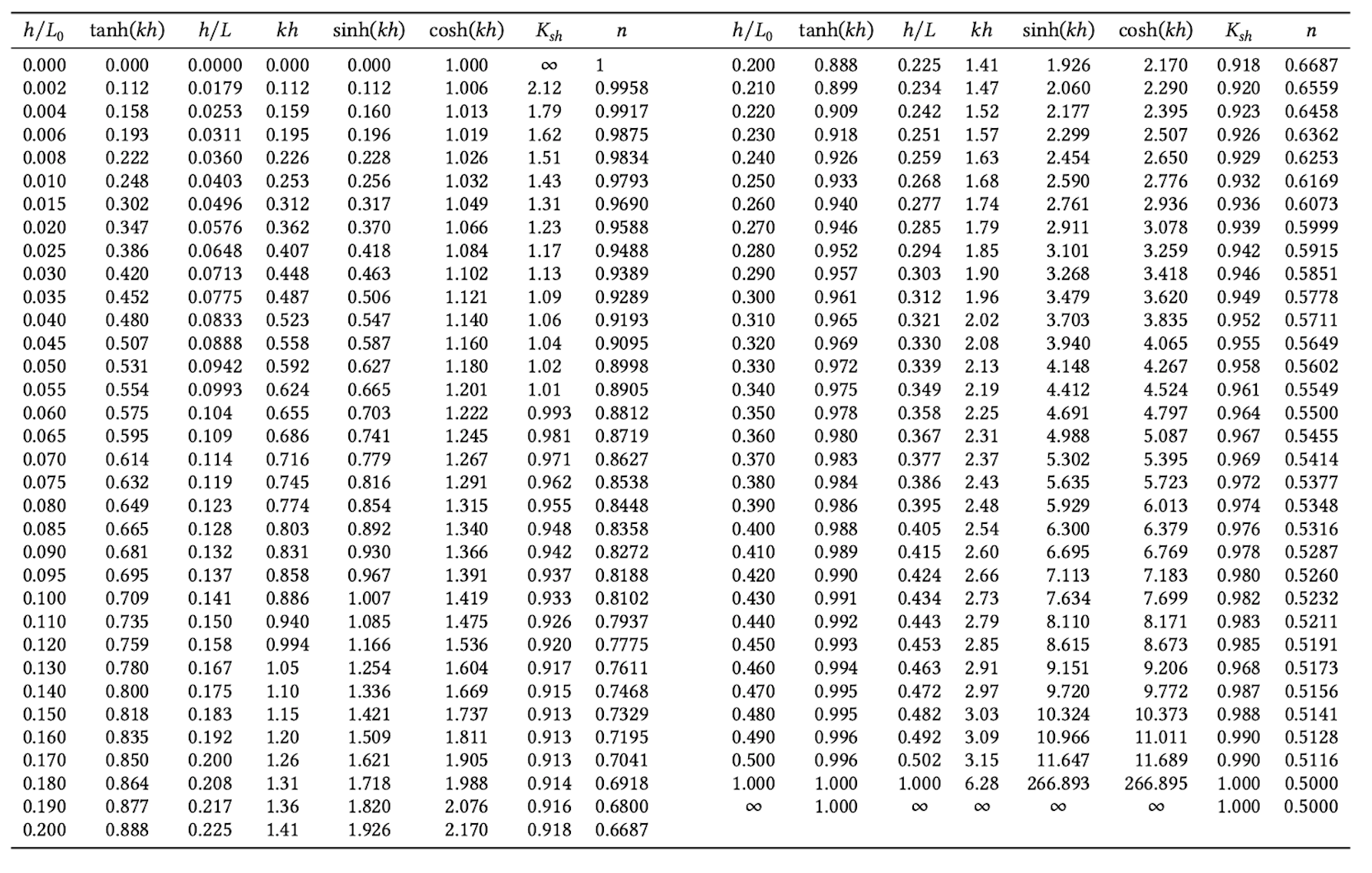
The dispersion relationship is implicit in terms of the wavenumber. This means that in order to solve the equation for transitional water depth an iterative process is required (to calculate \(L\) from given \(h\) and \(T\)). There are also explicit expressions available that approximate the solution closely. Alternatively, use can be made of a look-up table like Table A.3 that gives \(h/L\)for given \(h/L_0\) (with the deep water wavelength \(L_0 = gT^2/2\pi\)).
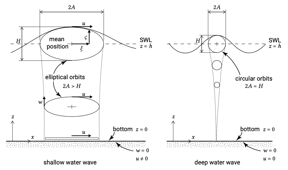
The water particle displacement is shown in Fig. A.2 for a wave in shallow water and for a wave in deep water. In deep water the wave motion does not extend down to the bed; in shallow water the water makes an oscillating movement over the entire depth. Near the surface the water particles describe an elliptical path; near the bottom the water particles make a horizontal oscillating movement.
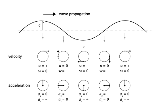
Figure A.3 shows the relation between the direction of the velocity and the acceleration of water particles at certain phases in the wave period.