
5.5.1: Wave-induced mass flux or momentum
- Page ID
- 16326

\( \newcommand{\vecs}[1]{\overset { \scriptstyle \rightharpoonup} {\mathbf{#1}} } \)
\( \newcommand{\vecd}[1]{\overset{-\!-\!\rightharpoonup}{\vphantom{a}\smash {#1}}} \)
\( \newcommand{\id}{\mathrm{id}}\) \( \newcommand{\Span}{\mathrm{span}}\)
( \newcommand{\kernel}{\mathrm{null}\,}\) \( \newcommand{\range}{\mathrm{range}\,}\)
\( \newcommand{\RealPart}{\mathrm{Re}}\) \( \newcommand{\ImaginaryPart}{\mathrm{Im}}\)
\( \newcommand{\Argument}{\mathrm{Arg}}\) \( \newcommand{\norm}[1]{\| #1 \|}\)
\( \newcommand{\inner}[2]{\langle #1, #2 \rangle}\)
\( \newcommand{\Span}{\mathrm{span}}\)
\( \newcommand{\id}{\mathrm{id}}\)
\( \newcommand{\Span}{\mathrm{span}}\)
\( \newcommand{\kernel}{\mathrm{null}\,}\)
\( \newcommand{\range}{\mathrm{range}\,}\)
\( \newcommand{\RealPart}{\mathrm{Re}}\)
\( \newcommand{\ImaginaryPart}{\mathrm{Im}}\)
\( \newcommand{\Argument}{\mathrm{Arg}}\)
\( \newcommand{\norm}[1]{\| #1 \|}\)
\( \newcommand{\inner}[2]{\langle #1, #2 \rangle}\)
\( \newcommand{\Span}{\mathrm{span}}\) \( \newcommand{\AA}{\unicode[.8,0]{x212B}}\)
\( \newcommand{\vectorA}[1]{\vec{#1}} % arrow\)
\( \newcommand{\vectorAt}[1]{\vec{\text{#1}}} % arrow\)
\( \newcommand{\vectorB}[1]{\overset { \scriptstyle \rightharpoonup} {\mathbf{#1}} } \)
\( \newcommand{\vectorC}[1]{\textbf{#1}} \)
\( \newcommand{\vectorD}[1]{\overrightarrow{#1}} \)
\( \newcommand{\vectorDt}[1]{\overrightarrow{\text{#1}}} \)
\( \newcommand{\vectE}[1]{\overset{-\!-\!\rightharpoonup}{\vphantom{a}\smash{\mathbf {#1}}}} \)
\( \newcommand{\vecs}[1]{\overset { \scriptstyle \rightharpoonup} {\mathbf{#1}} } \)
\( \newcommand{\vecd}[1]{\overset{-\!-\!\rightharpoonup}{\vphantom{a}\smash {#1}}} \)
\(\newcommand{\avec}{\mathbf a}\) \(\newcommand{\bvec}{\mathbf b}\) \(\newcommand{\cvec}{\mathbf c}\) \(\newcommand{\dvec}{\mathbf d}\) \(\newcommand{\dtil}{\widetilde{\mathbf d}}\) \(\newcommand{\evec}{\mathbf e}\) \(\newcommand{\fvec}{\mathbf f}\) \(\newcommand{\nvec}{\mathbf n}\) \(\newcommand{\pvec}{\mathbf p}\) \(\newcommand{\qvec}{\mathbf q}\) \(\newcommand{\svec}{\mathbf s}\) \(\newcommand{\tvec}{\mathbf t}\) \(\newcommand{\uvec}{\mathbf u}\) \(\newcommand{\vvec}{\mathbf v}\) \(\newcommand{\wvec}{\mathbf w}\) \(\newcommand{\xvec}{\mathbf x}\) \(\newcommand{\yvec}{\mathbf y}\) \(\newcommand{\zvec}{\mathbf z}\) \(\newcommand{\rvec}{\mathbf r}\) \(\newcommand{\mvec}{\mathbf m}\) \(\newcommand{\zerovec}{\mathbf 0}\) \(\newcommand{\onevec}{\mathbf 1}\) \(\newcommand{\real}{\mathbb R}\) \(\newcommand{\twovec}[2]{\left[\begin{array}{r}#1 \\ #2 \end{array}\right]}\) \(\newcommand{\ctwovec}[2]{\left[\begin{array}{c}#1 \\ #2 \end{array}\right]}\) \(\newcommand{\threevec}[3]{\left[\begin{array}{r}#1 \\ #2 \\ #3 \end{array}\right]}\) \(\newcommand{\cthreevec}[3]{\left[\begin{array}{c}#1 \\ #2 \\ #3 \end{array}\right]}\) \(\newcommand{\fourvec}[4]{\left[\begin{array}{r}#1 \\ #2 \\ #3 \\ #4 \end{array}\right]}\) \(\newcommand{\cfourvec}[4]{\left[\begin{array}{c}#1 \\ #2 \\ #3 \\ #4 \end{array}\right]}\) \(\newcommand{\fivevec}[5]{\left[\begin{array}{r}#1 \\ #2 \\ #3 \\ #4 \\ #5 \\ \end{array}\right]}\) \(\newcommand{\cfivevec}[5]{\left[\begin{array}{c}#1 \\ #2 \\ #3 \\ #4 \\ #5 \\ \end{array}\right]}\) \(\newcommand{\mattwo}[4]{\left[\begin{array}{rr}#1 \amp #2 \\ #3 \amp #4 \\ \end{array}\right]}\) \(\newcommand{\laspan}[1]{\text{Span}\{#1\}}\) \(\newcommand{\bcal}{\cal B}\) \(\newcommand{\ccal}{\cal C}\) \(\newcommand{\scal}{\cal S}\) \(\newcommand{\wcal}{\cal W}\) \(\newcommand{\ecal}{\cal E}\) \(\newcommand{\coords}[2]{\left\{#1\right\}_{#2}}\) \(\newcommand{\gray}[1]{\color{gray}{#1}}\) \(\newcommand{\lgray}[1]{\color{lightgray}{#1}}\) \(\newcommand{\rank}{\operatorname{rank}}\) \(\newcommand{\row}{\text{Row}}\) \(\newcommand{\col}{\text{Col}}\) \(\renewcommand{\row}{\text{Row}}\) \(\newcommand{\nul}{\text{Nul}}\) \(\newcommand{\var}{\text{Var}}\) \(\newcommand{\corr}{\text{corr}}\) \(\newcommand{\len}[1]{\left|#1\right|}\) \(\newcommand{\bbar}{\overline{\bvec}}\) \(\newcommand{\bhat}{\widehat{\bvec}}\) \(\newcommand{\bperp}{\bvec^\perp}\) \(\newcommand{\xhat}{\widehat{\xvec}}\) \(\newcommand{\vhat}{\widehat{\vvec}}\) \(\newcommand{\uhat}{\widehat{\uvec}}\) \(\newcommand{\what}{\widehat{\wvec}}\) \(\newcommand{\Sighat}{\widehat{\Sigma}}\) \(\newcommand{\lt}{<}\) \(\newcommand{\gt}{>}\) \(\newcommand{\amp}{&}\) \(\definecolor{fillinmathshade}{gray}{0.9}\)Propagating waves not only carry energy across the ocean surface but momentum as well. Momentum is defined as the product of mass and velocity. It can be thought of as mass in motion or a mass transport or flux: a water particle has a mass, and if the particle is moving it has momentum. Momentum per unit volume can thus be written as the product of the mass density \(\rho\) and the velocity \(\vec{u} = (u_x, u_y, w)\) of the water particles. Momentum (per unit volume) \(\rho \vec{u} = (\rho u_x, \rho u_y, \rho w)\) is a vector quantity, a quantity which is fully described by both magnitude and direction. The direction of the momentum vector is the same as the direction of the velocity vector.
The total amount of wave momentum per unit surface area in wave propagating direction is obtained by integration over the depth. Averaged over time this gives (with \(u\) the horizontal orbital velocity in the wave propagation direction):
\[q = \overline{\int_{-h}^{\eta} \rho u dz}\label{eq5.5.1.1}\]
There is only a contribution to the momentum from the wave trough level to the wave crest level, since below the wave trough the velocity varies harmonically in time (see Sect. 5.4.1), giving a zero time-averaged result. If we measure the velocity at some point above MSL we will only record velocities during part of the wave period and all of the recordings will be positive (and in the wave propagation direction). Between the wave trough level and MSL we will record velocities for a larger part of the wave period and although a part of the recording will be negative, the wave-averaged mean velocity will still be positive. The momentum \(q\) can thus be interpreted as a net flux of mass between wave trough and wave crest associated with wave propagation.
We can compute the integral of Eq. \(\ref{eq5.5.1.1}\) for a single harmonic component (non-breaking) by substituting the velocity according to linear wave theory (see Eq. 5.4.1.1) at \(z = 0\) and integrating from \(z = 0\) to the instantaneous surface elevation \(\eta = a \cos \omega t\). We then find for the mean momentum in a plane perpendicular to the wave propagation direction per unit surface area:
\[q_{\text{non-breaking}} = \overline{\int_0^{a \cos \omega t} \rho \dfrac{a \omega}{\tanh kh} \cos \omega t dz} = \overline{a \cos \omega t \rho \dfrac{a \omega}{\tanh kh} \cos \omega t} = \dfrac{\rho a^2 \omega}{2\tanh kh} = \dfrac{\rho g a^2}{2c} = \dfrac{E}{c}\label{eq5.5.1.2}\]
This expression shows that \(q\) is a non-linear quantity in the amplitude \(a\). The result is valid to second-order accuracy in the amplitude (linear wave theory is first order). Apparently, wave-induced mass flux occurs even for a perfect sinusoidal orbital motion, but is a second-order effect. In the linear, small amplitude approximation, \(q\) is zero and wave propagation is merely a matter of movement of the wave form, not of mass. In relation to net mass flux associated with wave propagation the term Stokes’ drift is often used (see Intermezzo 5.3).
Equation \(\ref{eq5.5.1.2}\) is valid outside the surf zone. In the surf zone the mass flux is substantially larger than outside the surf zone. It is assumed to consist of two parts, one due to the progressive character of the waves (Eq. \(\ref{eq5.5.1.2}\)) and the other due to the surface roller in breaking waves:
\[q_{\text{drift}} = q_{\text{non-breaking}} + q_{\text{roller}} = \dfrac{E}{c} + \dfrac{\alpha E_r}{c}\label{eq5.5.1.3}\]
In this equation, \(E_r\) is the roller energy. The first part of the right hand side is the mass flux for non-breaking waves, whereas the second part accounts for the contribution of the mass of the surface roller. Various authors have argued values for the factor \(\alpha\) in Eq. \(\ref{eq5.5.1.3}\) to be in the range of 0.22 to 2 (Nairn et al., 1990; Roelvink & Stive, 1989). Their arguments are too involved to treat in this course and here we assume that \(\alpha\) is order 1.
In the case of a closed boundary like a coastline, there is a zero net mass transport through the vertical as otherwise water will increasingly pile up against the coast. This means that there must be a net velocity below the wave trough level to compensate for the flux above the wave trough level: a return current. The cross-shore depth-mean velocity below the wave trough level must compensate for the mass flux perpendicular to the shore and is therefore given by:
\[U_{\text{below through}} = -\dfrac{q_{\text{drift}, x}}{\rho h} = -\dfrac{q_{\text{drift}} \cos \theta}{\rho h}\]
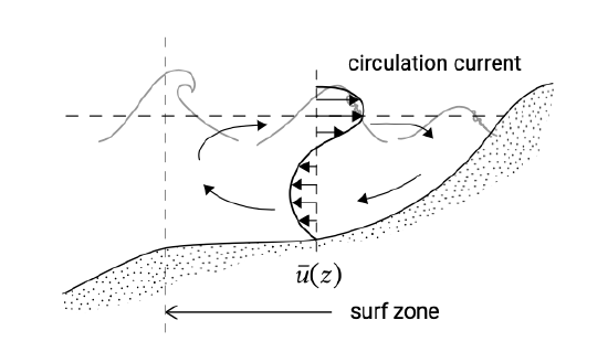
In breaking waves, the mass transport towards the coast between wave crest and wave trough may be quite large, resulting in rather large seaward directed velocities under the wave trough level (see Fig. 5.25). The large return current in the surf zone is called undertow.
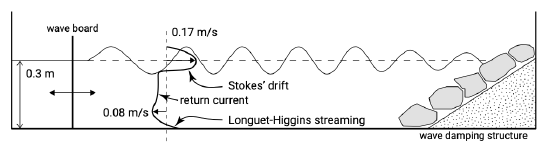
Also in the two dimensional case of a laboratory wave flume, the same mass of water has to return to the ‘sea’ again. In the lower part of the water column this gives a return flow (see Fig. 5.26). The figure also shows the Longuet-Higgins streaming close to the bed (see Sect. 5.4.3). In Fig. 5.25, we have assumed that in the surf zone the steady Longuet-Higgins streaming may well be overridden by the undertow. The distribution over the depth of the return current or undertow (and the streaming) can be solved using a horizontal momentum equation (not depth-averaged!), see Sect. 5.5.6.
Appendix B provides an example of wave flume experiments of periodic and random waves on a gently sloping beach (Stive, 1985). Figure B.2 shows the measurements of return currents in shoaling and breaking periodic waves. In non-breaking waves there is relatively small return current. In breaking waves, the mass transport towards the coast between wave crest and wave trough may be quite large, resulting in rather large seaward directed time-mean velocities under the wave trough level.
We explained mass transport from an Eulerian point of view in the text above (by placing a measuring pole in a fixed cross-section and concluding that above the wave trough level the recorded velocity has a non-zero time-averaged result in the wave propagation direction). It can also be explained from a Lagrangian point of view, viz. by following a water particle moving in its orbital motion (see Fig. 5.20). Since the horizontal movement is in general smaller closer to the bed (see Eq. 5.22 and Fig. 5.21), the water particle moves faster in the wave propagation direction when it is located under the wave crest, than it runs backward when under the trough of the wave. As a result particle paths are not entirely closed orbits and there is a residual motion in the wave propagation direction over one wave period. This residual motion is referred to as Stokes’ drift and gives rise to a net mass transport in the direction of wave propagation. When we integrate the Lagrangian mass transport over the vertical we get the same result as the Eulerian mass transport above the wave trough level.
The undertow is important for seaward sediment transport because of the relatively high offshore-directed velocity in the lower and middle part of the water column in a zone with relatively high sediment concentrations (due to wave breaking). The undertow is thought to be responsible for the severe beach erosion during heavy storms. Sediment transport due to return currents is also important for shallow areas that have a deeper area between them and the coast. Examples are shallow areas on the ebb-tidal deltas of coastal inlet systems, where the mass flux is not (entirely) compensated by undertow as the water can flow away at the back of these flats (where often tidal channels are present). This is further discussed in Sect. 9.4.1.