
7.5.2: Decomposition of the transport rate
- Page ID
- 16379

\( \newcommand{\vecs}[1]{\overset { \scriptstyle \rightharpoonup} {\mathbf{#1}} } \)
\( \newcommand{\vecd}[1]{\overset{-\!-\!\rightharpoonup}{\vphantom{a}\smash {#1}}} \)
\( \newcommand{\id}{\mathrm{id}}\) \( \newcommand{\Span}{\mathrm{span}}\)
( \newcommand{\kernel}{\mathrm{null}\,}\) \( \newcommand{\range}{\mathrm{range}\,}\)
\( \newcommand{\RealPart}{\mathrm{Re}}\) \( \newcommand{\ImaginaryPart}{\mathrm{Im}}\)
\( \newcommand{\Argument}{\mathrm{Arg}}\) \( \newcommand{\norm}[1]{\| #1 \|}\)
\( \newcommand{\inner}[2]{\langle #1, #2 \rangle}\)
\( \newcommand{\Span}{\mathrm{span}}\)
\( \newcommand{\id}{\mathrm{id}}\)
\( \newcommand{\Span}{\mathrm{span}}\)
\( \newcommand{\kernel}{\mathrm{null}\,}\)
\( \newcommand{\range}{\mathrm{range}\,}\)
\( \newcommand{\RealPart}{\mathrm{Re}}\)
\( \newcommand{\ImaginaryPart}{\mathrm{Im}}\)
\( \newcommand{\Argument}{\mathrm{Arg}}\)
\( \newcommand{\norm}[1]{\| #1 \|}\)
\( \newcommand{\inner}[2]{\langle #1, #2 \rangle}\)
\( \newcommand{\Span}{\mathrm{span}}\) \( \newcommand{\AA}{\unicode[.8,0]{x212B}}\)
\( \newcommand{\vectorA}[1]{\vec{#1}} % arrow\)
\( \newcommand{\vectorAt}[1]{\vec{\text{#1}}} % arrow\)
\( \newcommand{\vectorB}[1]{\overset { \scriptstyle \rightharpoonup} {\mathbf{#1}} } \)
\( \newcommand{\vectorC}[1]{\textbf{#1}} \)
\( \newcommand{\vectorD}[1]{\overrightarrow{#1}} \)
\( \newcommand{\vectorDt}[1]{\overrightarrow{\text{#1}}} \)
\( \newcommand{\vectE}[1]{\overset{-\!-\!\rightharpoonup}{\vphantom{a}\smash{\mathbf {#1}}}} \)
\( \newcommand{\vecs}[1]{\overset { \scriptstyle \rightharpoonup} {\mathbf{#1}} } \)
\( \newcommand{\vecd}[1]{\overset{-\!-\!\rightharpoonup}{\vphantom{a}\smash {#1}}} \)
\(\newcommand{\avec}{\mathbf a}\) \(\newcommand{\bvec}{\mathbf b}\) \(\newcommand{\cvec}{\mathbf c}\) \(\newcommand{\dvec}{\mathbf d}\) \(\newcommand{\dtil}{\widetilde{\mathbf d}}\) \(\newcommand{\evec}{\mathbf e}\) \(\newcommand{\fvec}{\mathbf f}\) \(\newcommand{\nvec}{\mathbf n}\) \(\newcommand{\pvec}{\mathbf p}\) \(\newcommand{\qvec}{\mathbf q}\) \(\newcommand{\svec}{\mathbf s}\) \(\newcommand{\tvec}{\mathbf t}\) \(\newcommand{\uvec}{\mathbf u}\) \(\newcommand{\vvec}{\mathbf v}\) \(\newcommand{\wvec}{\mathbf w}\) \(\newcommand{\xvec}{\mathbf x}\) \(\newcommand{\yvec}{\mathbf y}\) \(\newcommand{\zvec}{\mathbf z}\) \(\newcommand{\rvec}{\mathbf r}\) \(\newcommand{\mvec}{\mathbf m}\) \(\newcommand{\zerovec}{\mathbf 0}\) \(\newcommand{\onevec}{\mathbf 1}\) \(\newcommand{\real}{\mathbb R}\) \(\newcommand{\twovec}[2]{\left[\begin{array}{r}#1 \\ #2 \end{array}\right]}\) \(\newcommand{\ctwovec}[2]{\left[\begin{array}{c}#1 \\ #2 \end{array}\right]}\) \(\newcommand{\threevec}[3]{\left[\begin{array}{r}#1 \\ #2 \\ #3 \end{array}\right]}\) \(\newcommand{\cthreevec}[3]{\left[\begin{array}{c}#1 \\ #2 \\ #3 \end{array}\right]}\) \(\newcommand{\fourvec}[4]{\left[\begin{array}{r}#1 \\ #2 \\ #3 \\ #4 \end{array}\right]}\) \(\newcommand{\cfourvec}[4]{\left[\begin{array}{c}#1 \\ #2 \\ #3 \\ #4 \end{array}\right]}\) \(\newcommand{\fivevec}[5]{\left[\begin{array}{r}#1 \\ #2 \\ #3 \\ #4 \\ #5 \\ \end{array}\right]}\) \(\newcommand{\cfivevec}[5]{\left[\begin{array}{c}#1 \\ #2 \\ #3 \\ #4 \\ #5 \\ \end{array}\right]}\) \(\newcommand{\mattwo}[4]{\left[\begin{array}{rr}#1 \amp #2 \\ #3 \amp #4 \\ \end{array}\right]}\) \(\newcommand{\laspan}[1]{\text{Span}\{#1\}}\) \(\newcommand{\bcal}{\cal B}\) \(\newcommand{\ccal}{\cal C}\) \(\newcommand{\scal}{\cal S}\) \(\newcommand{\wcal}{\cal W}\) \(\newcommand{\ecal}{\cal E}\) \(\newcommand{\coords}[2]{\left\{#1\right\}_{#2}}\) \(\newcommand{\gray}[1]{\color{gray}{#1}}\) \(\newcommand{\lgray}[1]{\color{lightgray}{#1}}\) \(\newcommand{\rank}{\operatorname{rank}}\) \(\newcommand{\row}{\text{Row}}\) \(\newcommand{\col}{\text{Col}}\) \(\renewcommand{\row}{\text{Row}}\) \(\newcommand{\nul}{\text{Nul}}\) \(\newcommand{\var}{\text{Var}}\) \(\newcommand{\corr}{\text{corr}}\) \(\newcommand{\len}[1]{\left|#1\right|}\) \(\newcommand{\bbar}{\overline{\bvec}}\) \(\newcommand{\bhat}{\widehat{\bvec}}\) \(\newcommand{\bperp}{\bvec^\perp}\) \(\newcommand{\xhat}{\widehat{\xvec}}\) \(\newcommand{\vhat}{\widehat{\vvec}}\) \(\newcommand{\uhat}{\widehat{\uvec}}\) \(\newcommand{\what}{\widehat{\wvec}}\) \(\newcommand{\Sighat}{\widehat{\Sigma}}\) \(\newcommand{\lt}{<}\) \(\newcommand{\gt}{>}\) \(\newcommand{\amp}{&}\) \(\definecolor{fillinmathshade}{gray}{0.9}\)As explained in Ch. 5, the velocity \(u\) close to the bed can be assumed to consist of a wave group averaged component \(\bar{u}\), a short wave averaged oscillatory component \(u_{lo}\) and a short wave component \(u_{hi}\):
\[u = \underbrace{\bar{u}}_{\begin{array} {c} {\text{time-mean component}} \\ {\text{(streaming outside surf zone,}} \\ {\text{undertow in surf zone)}} \end{array}} + \underbrace{u_{lo}}_{\begin{array} {c} {\text{low-frequency motion}} \\ {\text{at wave group scale}} \end{array}} + \underbrace{u_{hi}}_{\begin{array} {c} {\text{oscillatory motion}} \\ {\text{at short wave scale}} \end{array}}\]
We are now interested in the relative contributions of these components of the time-varying flow to the net sediment transport (net meaning averaged over the wave group). Let us for simplicity focus on the third odd velocity moment that determines the bed load transport (see Eq. 6.7.2.9 and 6.7.2.10). By assuming that \(\bar{u} \ll u_{lo} \ll u_{hi}\) and using a Taylor expansion (see Intermezzo 7.3), Roelvink and Stive (1989) showed that the most important contributions to the third odd velocity moment are given by:
\[\langle u|u|^2 \rangle = \underbrace{3 \langle \bar{u} |u_{hi}|^2 \rangle}_{1} + \underbrace{\langle u_{hi} |u_{hi}|^2 \rangle}_{2} + \underbrace{3 \langle u_{lo} |u_{hi}|^2 \rangle}_{3} + ... \label{eq7.5.2.2}\]
The term \(|u_{hi}|^2\) in all three terms reflects that the sediment load is stirred by short waves. The first term in the RHS of Eq. \(\ref{eq7.5.2.2}\) is related to the subsequent transport by the mean current. The mean current could be the onshore directed wave-induced near bed streaming in non-breaking waves (Sect. 5.4.3) or the offshore directed undertow in the surf zone (Sect. 5.5). The second term and the third term represent the contribution to the velocity moment (and hence the net transport) of the oscillatory part of the instantaneous velocity; the second term is related to the short wave skewness, whereas the third term is associated with the interaction between the long wave velocity and the short wave velocity variance (the latter will change periodically on the timescale of short wave groups).
The second term is zero for a completely symmetrical oscillating velocity signal. However, in shoaling waves the velocity signal becomes asymmetric about the horizontal axis (positively skewed, meaning \(\langle u^3 \rangle >0\), see Sect. 5.3). As a result the second term is non-zero and onshore directed. In Intermezzo 6.5, we explained this transport contribution as follows; the larger onshore peak velocities under the wave crests are more effective in stirring up sediment than the smaller offshore velocities under the wave troughs. The relation between the amount of sediment stirring and velocity is non-linear; a twice as high velocity stirs up (in this case) four times more sediment. The result is an onshore transport.
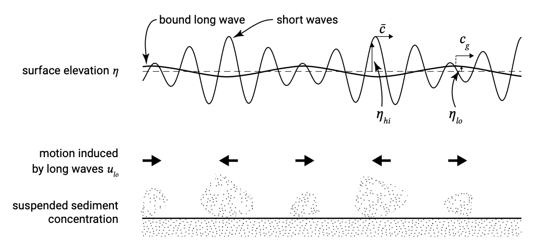
The third term is non-zero as long as there is a correlation between the slowly varying short wave velocity variance (the short wave envelope) and the long wave forced by the wave group. Outside the surf zone this correlation is negative (where the bound long wave is not yet ‘released from the group’); the mean water surface decrease (trough of the bound long wave) is found under the larger amplitude waves in the group (Fig. 7.20).
As long as the trough of the bound long wave coincides with the highest velocities in the group, most sediment is stirred up while the long wave velocities are offshore directed. The net transport by the bound long wave motion is therefore offshore directed (Fig. 7.20 shows this for suspended sediment transport). If the phase relationship between the short wave envelope and the long wave changes, this situation may change. The main reason why the phase relationship may change is that bound long waves become released during breaking of the short waves.
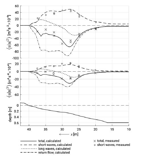
Roelvink and Stive (1989) analysed the decomposition of the velocity moments using laboratory measurements in a large (full-scale) wave flume. Calculated and measured total third and fourth odd flow moments (important for bed load and suspend load transport respectively) are compared in Fig. 7.21. The figure clearly shows the on-shore directed component due to short wave skewness. It increases in shoaling waves and decreases again in the surf zone (Sect. 5.3). The undertow component is offshore directed in the entire surf zone. The long wave contribution is offshore directed until the correlation between the short wave variance and long wave becomes positive somewhere in the surf zone.
From Fig. 7.21 it also becomes clear that the gross cross-shore transports are much higher than the net cross-shore transports. This makes accurate cross-shore transport predictions very difficult.
As mentioned in Sect. 7.5.1, during extreme conditions the transport contribution due to undertow is dominant. This explains that under higher and longer waves, as present during storms, a net offshore transport is observed, leading to a ‘winter’ profile (Sect. 7.3.3). By contrast, milder waves build up the profile to a ‘summer’ profile via onshore transport due to predominantly short wave skewness.
A similar decomposition of the transport rates can be made for the situation that tidal flow dominates the velocity \(u\). For this we refer to Sect. 9.7.2.