
7.5.3: Analytical solutions for the middle and lower shoreface
- Page ID
- 16380

\( \newcommand{\vecs}[1]{\overset { \scriptstyle \rightharpoonup} {\mathbf{#1}} } \)
\( \newcommand{\vecd}[1]{\overset{-\!-\!\rightharpoonup}{\vphantom{a}\smash {#1}}} \)
\( \newcommand{\id}{\mathrm{id}}\) \( \newcommand{\Span}{\mathrm{span}}\)
( \newcommand{\kernel}{\mathrm{null}\,}\) \( \newcommand{\range}{\mathrm{range}\,}\)
\( \newcommand{\RealPart}{\mathrm{Re}}\) \( \newcommand{\ImaginaryPart}{\mathrm{Im}}\)
\( \newcommand{\Argument}{\mathrm{Arg}}\) \( \newcommand{\norm}[1]{\| #1 \|}\)
\( \newcommand{\inner}[2]{\langle #1, #2 \rangle}\)
\( \newcommand{\Span}{\mathrm{span}}\)
\( \newcommand{\id}{\mathrm{id}}\)
\( \newcommand{\Span}{\mathrm{span}}\)
\( \newcommand{\kernel}{\mathrm{null}\,}\)
\( \newcommand{\range}{\mathrm{range}\,}\)
\( \newcommand{\RealPart}{\mathrm{Re}}\)
\( \newcommand{\ImaginaryPart}{\mathrm{Im}}\)
\( \newcommand{\Argument}{\mathrm{Arg}}\)
\( \newcommand{\norm}[1]{\| #1 \|}\)
\( \newcommand{\inner}[2]{\langle #1, #2 \rangle}\)
\( \newcommand{\Span}{\mathrm{span}}\) \( \newcommand{\AA}{\unicode[.8,0]{x212B}}\)
\( \newcommand{\vectorA}[1]{\vec{#1}} % arrow\)
\( \newcommand{\vectorAt}[1]{\vec{\text{#1}}} % arrow\)
\( \newcommand{\vectorB}[1]{\overset { \scriptstyle \rightharpoonup} {\mathbf{#1}} } \)
\( \newcommand{\vectorC}[1]{\textbf{#1}} \)
\( \newcommand{\vectorD}[1]{\overrightarrow{#1}} \)
\( \newcommand{\vectorDt}[1]{\overrightarrow{\text{#1}}} \)
\( \newcommand{\vectE}[1]{\overset{-\!-\!\rightharpoonup}{\vphantom{a}\smash{\mathbf {#1}}}} \)
\( \newcommand{\vecs}[1]{\overset { \scriptstyle \rightharpoonup} {\mathbf{#1}} } \)
\( \newcommand{\vecd}[1]{\overset{-\!-\!\rightharpoonup}{\vphantom{a}\smash {#1}}} \)
\(\newcommand{\avec}{\mathbf a}\) \(\newcommand{\bvec}{\mathbf b}\) \(\newcommand{\cvec}{\mathbf c}\) \(\newcommand{\dvec}{\mathbf d}\) \(\newcommand{\dtil}{\widetilde{\mathbf d}}\) \(\newcommand{\evec}{\mathbf e}\) \(\newcommand{\fvec}{\mathbf f}\) \(\newcommand{\nvec}{\mathbf n}\) \(\newcommand{\pvec}{\mathbf p}\) \(\newcommand{\qvec}{\mathbf q}\) \(\newcommand{\svec}{\mathbf s}\) \(\newcommand{\tvec}{\mathbf t}\) \(\newcommand{\uvec}{\mathbf u}\) \(\newcommand{\vvec}{\mathbf v}\) \(\newcommand{\wvec}{\mathbf w}\) \(\newcommand{\xvec}{\mathbf x}\) \(\newcommand{\yvec}{\mathbf y}\) \(\newcommand{\zvec}{\mathbf z}\) \(\newcommand{\rvec}{\mathbf r}\) \(\newcommand{\mvec}{\mathbf m}\) \(\newcommand{\zerovec}{\mathbf 0}\) \(\newcommand{\onevec}{\mathbf 1}\) \(\newcommand{\real}{\mathbb R}\) \(\newcommand{\twovec}[2]{\left[\begin{array}{r}#1 \\ #2 \end{array}\right]}\) \(\newcommand{\ctwovec}[2]{\left[\begin{array}{c}#1 \\ #2 \end{array}\right]}\) \(\newcommand{\threevec}[3]{\left[\begin{array}{r}#1 \\ #2 \\ #3 \end{array}\right]}\) \(\newcommand{\cthreevec}[3]{\left[\begin{array}{c}#1 \\ #2 \\ #3 \end{array}\right]}\) \(\newcommand{\fourvec}[4]{\left[\begin{array}{r}#1 \\ #2 \\ #3 \\ #4 \end{array}\right]}\) \(\newcommand{\cfourvec}[4]{\left[\begin{array}{c}#1 \\ #2 \\ #3 \\ #4 \end{array}\right]}\) \(\newcommand{\fivevec}[5]{\left[\begin{array}{r}#1 \\ #2 \\ #3 \\ #4 \\ #5 \\ \end{array}\right]}\) \(\newcommand{\cfivevec}[5]{\left[\begin{array}{c}#1 \\ #2 \\ #3 \\ #4 \\ #5 \\ \end{array}\right]}\) \(\newcommand{\mattwo}[4]{\left[\begin{array}{rr}#1 \amp #2 \\ #3 \amp #4 \\ \end{array}\right]}\) \(\newcommand{\laspan}[1]{\text{Span}\{#1\}}\) \(\newcommand{\bcal}{\cal B}\) \(\newcommand{\ccal}{\cal C}\) \(\newcommand{\scal}{\cal S}\) \(\newcommand{\wcal}{\cal W}\) \(\newcommand{\ecal}{\cal E}\) \(\newcommand{\coords}[2]{\left\{#1\right\}_{#2}}\) \(\newcommand{\gray}[1]{\color{gray}{#1}}\) \(\newcommand{\lgray}[1]{\color{lightgray}{#1}}\) \(\newcommand{\rank}{\operatorname{rank}}\) \(\newcommand{\row}{\text{Row}}\) \(\newcommand{\col}{\text{Col}}\) \(\renewcommand{\row}{\text{Row}}\) \(\newcommand{\nul}{\text{Nul}}\) \(\newcommand{\var}{\text{Var}}\) \(\newcommand{\corr}{\text{corr}}\) \(\newcommand{\len}[1]{\left|#1\right|}\) \(\newcommand{\bbar}{\overline{\bvec}}\) \(\newcommand{\bhat}{\widehat{\bvec}}\) \(\newcommand{\bperp}{\bvec^\perp}\) \(\newcommand{\xhat}{\widehat{\xvec}}\) \(\newcommand{\vhat}{\widehat{\vvec}}\) \(\newcommand{\uhat}{\widehat{\uvec}}\) \(\newcommand{\what}{\widehat{\wvec}}\) \(\newcommand{\Sighat}{\widehat{\Sigma}}\) \(\newcommand{\lt}{<}\) \(\newcommand{\gt}{>}\) \(\newcommand{\amp}{&}\) \(\definecolor{fillinmathshade}{gray}{0.9}\)Bowen (1980) derives expressions for the equilibrium shape of the middle and lower shoreface based on balancing onshore and offshore transport terms. He discusses the contribution of the main process of oscillatory orbital motion in combination with a mean flow, a higher harmonic orbital motion (asymmetry4) and a long (say bound) wave motion. Because of the non-linear coupling of these contributions in sediment
transport, their interactions are important. His analytical approach gives a good insight into these process interactions, and we note that the model efforts of Bailard (1981), Bailard and Inman (1981), Roelvink and Stive (1989) and Stive and De Vriend (1995) are very much inspired by this.
In this section, we present an abstracted form of certain parts of Bowen’s landmark paper.
Bowen starts by stating that:
“Any understanding of the relationship between the incident waves and the topography of a beach is greatly complicated by the beach being rarely, if ever, in equilibrium with the existing wave field. The morphology depends on some complex integral of past wave conditions, an integral heavily weighted towards periods of high waves. (...) The real situation is perhaps too complex for parameters to be developed without some guidance as to the relative importance of various possible processes. Simple theoretical models are particularly useful in defining these possibilities. (...) The purpose of the present paper is to develop a consistent model for onshore- offshore sediment transport under the influence of waves, currents and gravity. (...) The model is, however, neither unique nor necessarily correct (...), but a doubtful model is clearly preferable to no model. (...) The most important aspect of the present approach is the rigorous development of a theory, starting from any given model of sediment transport.”
Note that he speaks of a beach, but in what follows he concentrates rather on the middle and lower shoreface, not on the surf zone. The probable reason is that we lack straightforward analytical descriptions of the interactions between undertow, asymmetric oscillatory flow motion, breaking-induced turbulence and the bound and free long wave characteristics on the upper shoreface.
He explains the existence of a beach as follows:
“If a beach was exposed to waves having an exactly symmetrical, orbital velocity, all the sediment would slide down the slope and out to sea. The existence of the beach depends on small departures from symmetry in the velocity field balancing this tendency for gravity to move material offshore. (...) The development of the theory assumes as a basic hypothesis that the orbital motion of the incoming waves is the dominant motion.”
Hence, the basic idea is that the velocity \(u\) consists of two interacting components, the symmetrical orbital velocity \(U_0 = u_0 \cos (\omega t)\) and a perturbation \(U_1\) where:
\[u = U_0 + U_1,\ \ \text{ with generally} \ \ U_0 \gg U_1\]
The perturbation of the primary symmetrical harmonic can take many forms, where cases of particular interest are:
- A constant, steady current: \(U_1 = u_1\);
- The velocity field associated with a higher harmonic of the incoming wave: \(U_1 = u_m \cos (m \omega t + \theta_m)\), with \(m = 2, 3, 4, ...\);
- A perturbation due to a wave with a frequency \(\omega_t\) unrelated to \(\omega\): \(U_1 = u_t \cos (\omega_t t)\).
Note that in principle the steady current can be any current. Especially relevant for the shoreface is undertow in the surf zone and boundary layer streaming further offshore. The higher harmonics are relevant in the surf zone, with forward pitching or even sawtooth waves and \(\theta_m\) is non-zero, while further offshore we have just skewed or peaked waves (symmetrical around the vertical) where \(\theta_m\) is zero. We leave the case of the third bullet (a wave with a frequency unrelated to the primary harmonic) outside our discussion in these lecture notes.
Bowen adopts Bagnold’s transport description for uniform flow and transforms it for non-linear oscillatory motion, resulting in Eqs. 6.7.2.4 and 6.7.2.5. According to Bowen, Bagnold’s energetics model is the simplest available model that includes the basic properties that are necessary to describe cross-shore sediment transport. He especially stresses the explicit inclusion of the gravitational effect of a sloping bed.
Bowen also discusses the limitations of the energetics model:
“First, and perhaps most serious, the transport in this model depends only on the immediate flow conditions, adjusting instantaneously to changes without any time lag. Second, the theory applies to fully developed flow and does not describe initiation of movement; it does not apply to large particles that may move only intermittently at peak flows.”
First Bowen looked at suspended sediment transport and then at bed load transport both on the middle and lower shoreface. We will only repeat his suspended sediment transport derivations, because Stive and De Vriend (1995) showed by evaluating the transport terms for a typical shoreface situation that this transport mechanism is dominant on the middle and lower shoreface.
From Eq. 6.7.2.5, the suspended load transport can be expressed as:
\[I_s = \dfrac{\varepsilon_s c_f \rho}{w_s} \dfrac{u^3|u|}{(1 - \gamma u)} \ \text{ with } \ \gamma = \dfrac{\tan \alpha}{w_s}\label{eq7.5.3.2}\]
For normal transport conditions \(\gamma u < 1\). If \(\gamma u\) goes to 1, \(I_s\) goes to infinity and auto-suspension effects (avalanching, i.e. the slope is so steep that all particles go into suspension) totally dominate the transport.
Bowen now expands Eq. \(\ref{eq7.5.3.2}\), using the Taylor series as in Intermezzo 7.3, and takes a time-average (denoted by the overbar), arriving at a net transport \(\langle I_s \rangle\) over a number of wave periods. If we consider normal transport conditions, the expansion involves the small quantities \(U_1/U_0\) and \(\gamma U_0\). To second order, Bowen’s transport formulation reads:
\[\begin{array} {rcl} {rcl} {\langle I_s \rangle} & = & {\dfrac{\varepsilon_s c_f \rho}{w_s} [\overline{U_0^3 |U_0|} + \overline{4U_1 U_0^2 |U_0|} + \overline{6U_1^2 U_0 |U_0|} +} \\ {} & \ & {\gamma \left (\overline{U_0^4 |U_0|} + \overline{5U_1 U_0^3 |U_0|} \right ) + \gamma^2 \overline{U_0^5 |U_0|} + ...]} \end{array}\]
Terms of the form \(U_0^n |U_0|\) vanish if \(n\) is odd since \(U_0\) is assumed to be a symmetric oscillation.
Now, to first order, the equation reduces to:
\[\langle I_s \rangle = \dfrac{\varepsilon_s c_f \rho}{w_s} \left [\overline{4U_1 U_0^2 |U_0|} + \gamma \overline{U_0^4 |U_0|} + ... \right ]\label{eq7.5.3.4}\]
The first term describes the transport, onshore or offshore, due to a perturbation of the flow field \(U_1\). The second term involves the slope \(\tan \alpha\) and is generally positive, representing the tendency for downslope transport.
Bowen continues by evaluating the transport relations for the first form of the perturbation \(U_1\), viz. \(U_1 = u_1\) is a constant in time. Using Eq. \(\ref{eq7.5.3.4}\), this yields to first order:
\[\langle I_s \rangle = \dfrac{\varepsilon_s c_f \rho}{w_s} \left [\dfrac{16}{3\pi} u_1 u_0^3 + \dfrac{16}{15 \pi} \gamma u_0^5 \right ] \label{eq7.5.3.5}\]
Equation \(\ref{eq7.5.3.5}\) is a general result for any distribution of a steady flow \(U_1 (x)\). One could consider undertow, upwelling or downwelling but Bowen chooses to continue with boundary layer streaming as the relevant effect, which we support for the middle and lower shoreface.
An equilibrium profile, purely in suspended load, exists if the gravitational effects balance the influence of the steady current everywhere and \(\langle I_s \rangle\) vanishes. From Eq. \(\ref{eq7.5.3.5}\), when \(\langle I_s \rangle = 0\):
\[\gamma = \dfrac{\tan \alpha}{w_s} = - \dfrac{5u_1}{u_0^2}\]
This relationship essentially contains no free parameters, which is an attractive feature of Bagnold’s model.
The second-order, Eulerian mean velocity due to boundary layer streaming is of order \(-u_0^2/c\) (Eq. 5.4.3.3), where \(c\) is the wave phase speed (Eq. 3.5.2.2), so that:
\[\tan \alpha \simeq \dfrac{5w_s}{c} = \dfrac{5w_s \omega}{g \tanh kh}\label{eq7.5.3.7}\]
where \(k\) is the local wavenumber, \(h\) the water depth. This yields an expression for the equilibrium slope in terms of \(w_s \omega /g\), a dimensionless parameter also used by Dean (1973).
If sediment of a given grain size is in equilibrium with the local slope so that \(\langle I_s \rangle\) vanishes for this grain size, any coarser material with a larger fall velocity has a smaller value of \(\gamma\). The term involving gravity is reduced, the onshore term remains constant,
coarser material therefore moves onshore; similarly, finer material moves offshore as observed. As can be observed from Eq. \(\ref{eq7.5.3.7}\), profiles of coarser material are steeper, any material that finds itself on a beach that is ‘too steep’ moves seawards. This leads to a new null-point hypothesis that is in far better agreement with observations than classical models.
In shallow water \(c\) tends to \(\sqrt{gh}\) and Eq. \(\ref{eq7.5.3.7}\) is readily integrated:
\[\tan \alpha = \dfrac{dh}{dx} = 5w_s / \sqrt{gh} \Rightarrow h^3 \simeq (7.5 w_s x)^2/g\]
And thus the equilibrium profile is described by:
\[h \simeq (7.5 w_s)^{2/3} /g^{1/3} x^{2/3}\label{eq7.5.3.9}\]
Intriguingly, this result accurately resembles the earlier presented results for the equilibrium shoreface profiles of Bruun and Dean (Eq. 7.2.2.1). The profile shape factor \(A\) according to Eq. \(\ref{eq7.5.3.9}\) is for \(w_s = 0.0256\ m/s\):
\[A = (7.5 w_s)^{2/3} / g^{1/3} = 0.16\]
This result is reasonably close to \(A = 0.10\) for the same fall velocity according to Eq. 7.2.2.7.
Next, Bowen considered the role of the higher harmonics associated with the incoming wave field (thus, wave asymmetry). The perturbation \(U_1\) now is a higher harmonic of \(U_0 = u_0 \cos (\omega t)\), viz. \(U_1 = u_m \cos (m \omega t + \theta_m)\).
The effect of wave asymmetry on the transport is derived from the first order expression Eq. \(\ref{eq7.5.3.4}\). The first order term \(4U_1 U_0^2 |U_0|\) vanishes if \(m\) is odd. We therefore only have to take even harmonics into account, the second harmonic (\(m = 2\)) being the most important. For the second harmonic we have:
\[4 \overline{U_1 |U_0^2| U_0} = -\dfrac{16}{5\pi} u_0^3 u_2 \cos \theta_2\label{eq7.5.3.11}\]
The term arising from Eq. \(\ref{eq7.5.3.11}\) is not an alternative to the contribution due to the Longuet-Higgins boundary layer streaming, but an additional factor. We therefore add the term from Eq. \(\ref{eq7.5.3.11}\) to Eq. \(\ref{eq7.5.3.5}\) and find:
\[\langle I_s \rangle = \dfrac{\varepsilon_s c_f \rho}{w_s} \dfrac{16}{15 \pi} u_0^3 [5u_1 - 3u_2 \cos \theta_2 + \gamma u_0^2]\]
Again, an equilibrium profile for suspended load is found for \(\langle I_s \rangle = 0\):
\[\gamma = \dfrac{\tan \alpha}{w_s} = -\dfrac{5u_1}{u_0^2} + \dfrac{3u_2 \cos \theta_2}{u_0^2}\]
To evaluate this expression, Bowen assumed \(\theta_2 = 0\) and used the second order Stokes solution (see Intermezzo 5.1) to estimate \(u_2\). Herewith he derived that:
\[\tan \alpha \simeq \dfrac{9}{4} \dfrac{w_s}{c} [2 + (\sinh kh)^{-2}] \label{eq7.5.3.14}\]
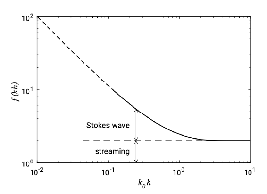
The term in brackets is shown in Fig. 7.22. In deep water, the effect of wave asymmetry is negligible compared to that of the wave boundary layer streaming. As the waves shoal, the wave harmonics become increasingly important. Since in very shallow water the Stokes solution is not necessarily a good approximation, the trend is indicated by a dashed line. At some point, the waves break and the form of \(u_2\) is only known from very limited empirical data.
According to Eq. \(\ref{eq7.5.3.14}\), wave asymmetry becomes as important as drift when:
\[\sinh kh \sim 2^{-1/2}\label{eq7.5.3.15}\]
\[h \sim 0.01 gT^2\label{eq7.5.3.16}\]
where \(T\) is the wave period. Equation \(\ref{eq7.5.3.15}\) and \(\ref{eq7.5.3.16}\) suggests that the extent of the nearshore area in which wave asymmetry is the dominant effect is strongly dependent on the period of the incoming waves. On the west coast of North America, which is generally exposed to waves of much longer periods, wave asymmetry should have a much more significant effect than on the east coast.
As \(kh\) becomes small, then from Eq. \(\ref{eq7.5.3.14}\) an expression for the equilibrium profile due to asymmetry can be derived, comparable to Eq. \(\ref{eq7.5.3.9}\):
\[h^5 \sim \left (\dfrac{5.7 w_s x}{\omega^2} \right )^2 g\]
Bowen’s landmark paper contains many more interesting analytical derivations and again we note that these analytical ideas have been at the basis of many numerical process-based model efforts. It is a paper worth studying if one is interested in solving the cross-shore morphology problem.
Bowen (1980) outlined a Taylor series expansion of the velocity moment \(u^n |u|\). He assumed the velocity \(u\) to consist of two interacting components, viz. \(U_0\) and a perturbation \(U_1\), hence \(u = U_0 + U_1\). Under the assumption that \(U_0\) is much larger than \(U_1\), the Taylor series expansion reads:
\[u^n |u| = U_0^n |U_0| + (n + 1) U_1 U_0^{n - 1} |U_0| + \dfrac{n(n + 1)}{2} U_1^2 U_0^{n - 2} |U_0| + ...\]
In practice, \(U_0\) is the wave orbital velocity \(U_0 = u_0 \cos (\omega t)\) which vanishes during the orbital cycle, and the assumption that \(U_1\) is small compared to \(U_0\) is not justified during the stages of the orbital velocity when \(U_0\) is small. The approximation is really that \(U_1 \ll u_0\), the maximum orbital velocity, and that the significant periods for transport are when \(U_0\) is large. This is probably a reasonable assumption as the transport goes as the third or fourth power of the total velocity.
4. In this section – as opposed to elsewhere in the book – we follow the wording of Bowen and use the word asymmetry for a skewed wave that is asymmetric about the vertical axis.