5.3: Wave asymmetry and skewness

In the previous sections linear wave propagation from deep to shallow water was discussed. We considered the propagation and conservation of a bulk quantity, the energy, in the shoaling region and breaker zone without considering any exchange of energy (or momentum) between different wave components due to non-linear interactions. The local wave characteristics were described by linear wave theory.

However, waves propagating towards the shore become more and more asymmetric until the point of wave breaking. Besides an increase in wave height, the shoaling process is typically characterised by:

• gradual peaking of the wave crest and a flattening of the trough (this asymmetry relative to the horizontal axis is called skewness);
• relative steepening of the face until breaking occurs, resulting in a pitched-forward wave shape (this asymmetry relative to the vertical axis is often simply called asymmetry).

These non-linear effects cannot be described by linear theory and the closer we come to the shore the more apparent the deviations from linear theory become. Numerous non-linear theories (Stokes theory, cnoidal wave theory, Boussinesq equations, see Intermezzo 5.1 for an overview) have been developed to take into account the complicated non-linear processes. The non-linear effects are crucial in determining the magnitude of the wave-induced transport (see Ch. 7). In the following we will there- fore subsequently consider skewness and asymmetry.

Skewness

Figure 5.12: A skewed wave (\(H/h = 0.5\) and \(L/h = 30\)) with on the horizontal axis the phase \(S(x, t) = \omega t - kx\). The shallow water wave is computed using 5^th order cnoidal wave theory (Intermezzo 5.1). Alternatively, it can be computed using a Fourier approximation, for which 20 harmonic components are required to converge towards the cnoidal solution (see Fig. 5.18). Produced using software by Fenton (https://johndfenton.com/Steady-waves/Fourier.html).

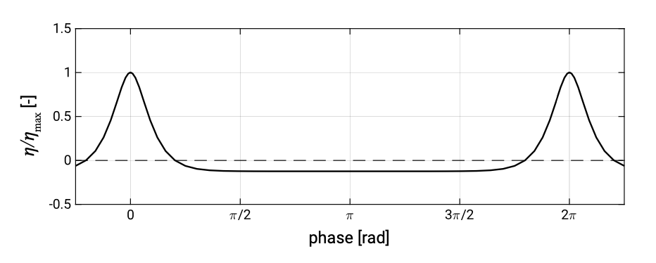
Figure 5.12 shows a wave with a long, flat trough and narrow, peaked crest, as can be observed in shallow water.

This asymmetric profile (relative to the horizontal axis) can only be described by a sum of sinusoidal waves with higher harmonics (frequencies that are a multiple of the basis frequency: \(\cos S, \cos 2S\) etc. with \(S = \omega t - kx\)). Let us illustrate this using Stokes 2^nd order theory. The second order expression for the surface elevation can be written as:

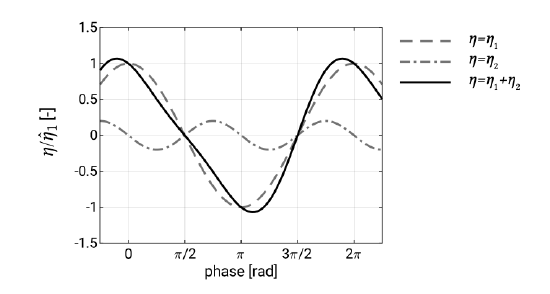
\[\eta = \hat{\eta}_1 \cos (\omega t - kx) + \hat{\eta}_2 \cos 2 (\omega t - kx)\label{eq5.3.1}\]

Figure 5.13: A second order Stokes’ wave (solid line) is composed of a first order (dashed line) and a second order (dashed-dotted line) component, according to Eq. \(\ref{eq5.3.1}\) with \(\hat{\eta}_2/\hat{\eta}_1 = 0.2\). The phase on the horizontal axis is the phase \(S = \omega t - kx\) of the primary harmonic. For more background on Stokes’ theory see Section 5.6.2 in Holthuijsen (2007).

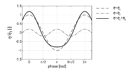
The amplitude of the second order correction is small compared to the first order component (as long as \(\hat{\eta}_1 = a\) is sufficiently small). The Stokes wave is sketched in Fig. 5.13.

It can be seen that the resulting Stokes wave profile \(\eta_1 + \eta_2\) has crests which are nar- rower and more peaked than those of a cosine profile and troughs that are wider and flatter; the profile is skewed. The second term \(\eta_2\) represents the Stokes second-order

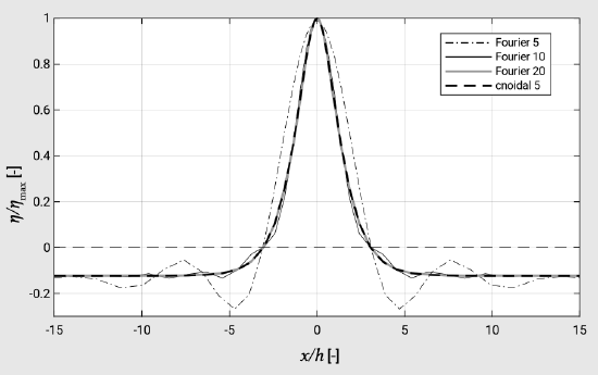
wave travelling at the same speed as the first-order wave \(\eta_1\) (hence, it does not obey the linear dispersion relation). Since the two components travel at the same speed the wave form does not change; it has a permanent form. Similarly in energy spectra of shoaling waves one can find harmonics of the spectral peak which are coherent in phase with the spectral peak. Note that taking into account higher order terms in Eq. \(\ref{eq5.3.1}\) will make the profile approach the profile of Fig. 5.12 more and more (see also Fig. 5.18).

Since the higher harmonics remain phase-locked and in phase with the primary harmonic, Stokes waves have a permanent form. This is different from the deep water situation we described in Ch. 3. There we considered the irregular sea state at a certain location to be the sum of linear, freely moving waves with random phases. Because of the different phase speeds of the different components (satisfying the linear dispersion relation) we could not have a permanent form.

Figure 5.14: Quantity of \(\eta^3 /\hat{\eta}_1^3\) compared to \(\eta /\hat{\eta}_1\) for a sinusoidal wave (left) and a second order Stokes wave (right) as a function of the phase \(S = \omega t - kx\) of the first or primary harmonic. Note that for the sinusoidal wave, the time-average \(\langle \eta^3 \rangle = 0\), whereas for the second order Stokes wave \(\langle \eta^3 \rangle > 0\).

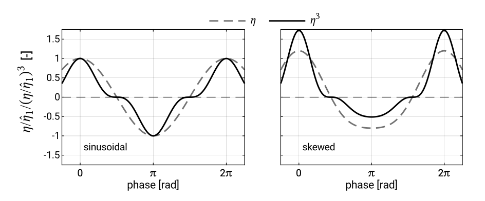
A statistical indicator for the skewness is the normalised cube of the surface elevation \(\langle \eta^3 \rangle /\sigma^3\): the time-averaged value of the cube of surface elevation normalised with the cube of the standard deviation \(\sigma^3\). The brackets denote time-averaging. Figure 5.14 shows the quantity \(\eta^3\) for a sinusoidal wave and for a 2^nd order Stokes wave. It can be seen that for a linear wave⁴ the time-averaged value \(\langle \eta^3 \rangle\) is zero, while for a Stokes wave it is not since the crests weigh more heavily than the troughs. The sign defines the ratio of crests to troughs. If it is positive – as is the case for the Stokes wave – then the crests are bigger than the troughs. Note that Stokes type wave forms have positive values of skewness, but zero asymmetry (around the vertical axis) since they are not pitched forward.

Linear theory could be used to estimate the variance (energy density) of nearshore waves. However, it cannot be used to estimate skewness since a linear superposition of random waves has by definition zero skewness over the ensemble.

Of course not only the surface elevation, but also the orbital velocities become skewed; the orbital velocities in the direction of wave movement (‘onshore’) become higher, and the orbital velocities against the wave direction (‘offshore’) become smaller. This naturally means that the duration of the onshore directed orbital motion becomes smaller and the duration of the offshore directed orbital signal becomes larger.

Asymmetry

Figure 5.15: Asymmetric wave (solid black line), computed as the superposition of a first order (dashed line) and a 90° forward phase-shifted second order signal (dashed-dotted line). The phase on the horizontal axis is the phase \(S = \omega t - kx\) of the first order component (or primary harmonic). The left figure shows the spatial variation at \(t = 0\) and the right figure shows the temporal variation of the water surface elevation at A (\(x/L = 0\)).

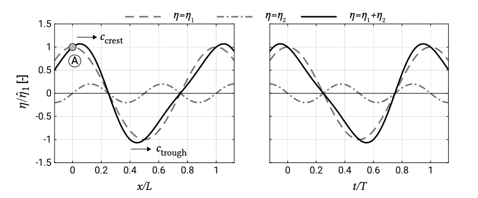
The pitched forward wave shape is the result of the fact that in shallow water the wave crest moves faster than the wave trough. This can be realised from the propagation speed of non-linear shallow water waves \(c = \sqrt{g(h + \eta)}\). Note that for small amplitude shallow water waves this reduces to \(c = \sqrt{gh}\) (see Intermezzo 3.5). The wave crest of a harmonic wave with amplitude \(a\) has a higher propagation velocity \(c_{\text{crest}} = \sqrt{g(h + a)}\) than the trough which propagates with \(c_{\text{through}} = \sqrt{g(h - a)}\). This leads to a pitched forward profile or relative steepening of the face of a wave that can be represented by the inclusion of a second harmonic that is forward phase-shifted with respect to the primary harmonic (see the left panel of Fig. 5.15). A Stokes wave train cannot exhibit wave asymmetry; because of the small amplitude approximation of the Stokes theory, the higher harmonic remains phase-locked to the primary harmonic. The right panel of Fig. 5.15 shows a time-series of a pitched forward (sawtooth-like) wave at one location, namely location A \((x/L = 0)\) in the left panel of Fig. 5.15.

The left panel of Fig. 5.15 shows a rapidly rising and slowly falling surface elevation. Note that for the sawtooth-like wave of Fig. 5.15, the phase shift between the first and the second harmonic is such that the asymmetry is maximum and the skewness is zero.

Figure 5.16: A 2^nd order asymmetric wave, generated using two harmonic components of which the second one is 90° forward phase-shifted.

The sawtooth-like wave of Fig. 5.15 can also be depicted as a function of \(S = \omega t - kx\). This results in Fig. 5.16. Compare this figure to the skewed wave of Fig. 5.13.

Figure 5.17: Quantity of \(\eta^3/\hat{\eta}_1^3\) compared to \(\eta /\hat{\eta}_1\) for a skewed wave (left) and an asymmetric wave (right). Note that for the skewed wave, the time-average \(\langle \eta^3 \rangle > 0\), whereas for the asymmetric wave \(\langle \eta^3 \rangle = 0\).

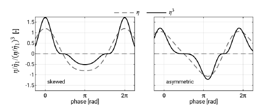
Figure 5.17 compares the quantity \(\eta^3\) for a skewed wave and an asymmetric wave as a function of the phase \(S = \omega t - kx\) of the first or primary harmonic. It can be seen that for the asymmetric wave the time-averaged value \(\langle \eta^3 \rangle \) is zero, while for the skewed wave it is not since the crests weigh more heavily than the troughs.

Shoaling waves first become gradually more skewed while remaining reasonably symmetric about the vertical axis – as an example see the flume measurements of Fig. B.2 in App. B. Closer to the surf zone, phase-shifting of the harmonic(s) leads to an increase in wave asymmetry and – eventually – to a decrease in wave skewness as well. Ultimately the pitching forward results in wave breaking.

The Ursell parameter \(U = HL^2/H^3\) can be used as an indicator for skewness and asymmetry. Doering and Bowen (1995) presented parameterisations of velocity skewness and asymmetry based on the Ursell parameter. They mainly focused on the skewness and asymmetry of the orbital velocities, because of their importance for sediment transport.

Intermezzo 5.1 Non-linear wave theories

Linear wave theory is obtained by linearising the free surface boundary conditions; the boundary conditions are applied to the mean water surface \(z = 0\) instead of the instantaneous water surface \(\eta\). Non-linearities can be neglected for not too steep waves in deep water (\(ak \ll 1\) for \(kh\) is large) or small amplitude waves in shallow water (\(a \ll h\) for \(kh\) is small).

Figure 5.18: Surface elevation records generated for \(H/h = 0.5\) and \(L/h = 30\), which amounts to \(T\sqrt{g/h} = 26.29\) or \(h/(gT^2) = 1.45 \times 10^{-3}\) and \(H/gT^2 = 7.23 \times 10^{-4}\) in Fig. 5.19. Both 5^th order cnoidal wave theory and a numerical Fourier approximation method (with 5, 10 and 20 harmonic components) are used. About 20 harmonic components are required for the Fourier approximation to converge towards the cnoidal solution. Produced using software by Fenton (https://johndfenton.com/Steady-waves/Fourier.html).

For a non-linear solution the free surface boundary conditions have to be applied at the free surface \(\eta\). The complication is that \(\eta\) is unknown. Amongst others the following non-linear theories have been developed:

• Stokes series expansion. Stokes used the result of the linear theory to find a first approximation to the neglected non-linear terms. This results in a second order correction to the first (linear) approximation of the solution. Note that the second order correction can be used to obtain a third order correction and so on. Non-linear terms consist of quadratic terms, so instead of the linear solution \(a \cos S\) (with the phase \(S = \omega t - kx\)), the 2^nd order solution has an additional term proportional to \(a^2 \cos^2 S\) that results in a term proportional to \(a^2 \cos 2S\), a harmonic with half the period of the linear solution. A Stokes series thus has the form \(\eta = \hat{\eta}_1 \cos S + \hat{\eta}_2 \cos 2S + \hat{\eta}_3 \cos 3S + ...\) in which the first term is the linear solution. For convergence, every next coefficient should be small compared to the lower-order coefficient, which will only be the case for sufficiently small amplitudes \(\hat{\eta}_1 = a\). Stokes theory does not converge in shallow water; if the Ursell parameter \(U = HL^2/h^3\) is too large the series diverges.
• The stream function theory is an alternative to the Stokes theory. It also adds higher harmonics to the linear solution.

Figure 5.19: The relative depth on the horizontal axis and the wave steepness on the vertical axis delineate the validity of various waves theories. The black dot indicates the wave of Fig. 5.18. (Based on Kamphuis, 2000; Le Méhauté, 1976).

• Applicable in shallow water is the cnoidal wave theory. Solutions are given in terms of elliptic integrals of the first kind; the solution in deep water is identical with linear wave theory and in shallow water to solitary wave theory. The latter is a single wave without a trough and a mass of water above mean water level moving entirely in the wave propagation direction.
• Boussinesq models can be seen as an extension of the shallow water equations (see for instance the DUT lecture notes CTB3350/CIE3310-09). The shallow water equations describe non-linear waves that all travel at the same speed \(c = \sqrt{g(h + \eta)}\). Orbital velocities are depth-uniform and the pressure is hydrostatic. Since there is no vertical variation of the wave field, the vertical does not have to be resolved. Boussinesq models account – to some extent – for the non-hydrostatic pressure distribution and depth-dependency of orbital velocities. The advantage over the shallow water equations is that Boussinesq models include frequency dispersion. Since the equations can still be integrated over the vertical, the equations are computationally efficient.

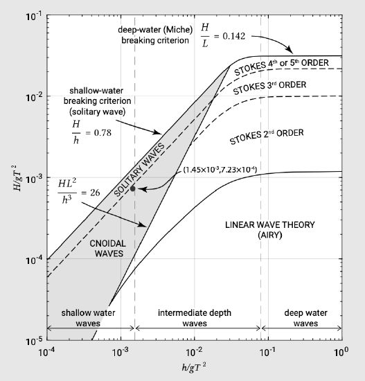
A review of the validity of various wave theories (until wave breaking) is given by Le Méhauté (1976). See also Fig. 5.19.

---

4. Similarly, in an irregular wave field approximated by a linear superposition of freely moving waves the skewness value is zero.