
6.6.1: General formulation
- Page ID
- 16357

\( \newcommand{\vecs}[1]{\overset { \scriptstyle \rightharpoonup} {\mathbf{#1}} } \)
\( \newcommand{\vecd}[1]{\overset{-\!-\!\rightharpoonup}{\vphantom{a}\smash {#1}}} \)
\( \newcommand{\dsum}{\displaystyle\sum\limits} \)
\( \newcommand{\dint}{\displaystyle\int\limits} \)
\( \newcommand{\dlim}{\displaystyle\lim\limits} \)
\( \newcommand{\id}{\mathrm{id}}\) \( \newcommand{\Span}{\mathrm{span}}\)
( \newcommand{\kernel}{\mathrm{null}\,}\) \( \newcommand{\range}{\mathrm{range}\,}\)
\( \newcommand{\RealPart}{\mathrm{Re}}\) \( \newcommand{\ImaginaryPart}{\mathrm{Im}}\)
\( \newcommand{\Argument}{\mathrm{Arg}}\) \( \newcommand{\norm}[1]{\| #1 \|}\)
\( \newcommand{\inner}[2]{\langle #1, #2 \rangle}\)
\( \newcommand{\Span}{\mathrm{span}}\)
\( \newcommand{\id}{\mathrm{id}}\)
\( \newcommand{\Span}{\mathrm{span}}\)
\( \newcommand{\kernel}{\mathrm{null}\,}\)
\( \newcommand{\range}{\mathrm{range}\,}\)
\( \newcommand{\RealPart}{\mathrm{Re}}\)
\( \newcommand{\ImaginaryPart}{\mathrm{Im}}\)
\( \newcommand{\Argument}{\mathrm{Arg}}\)
\( \newcommand{\norm}[1]{\| #1 \|}\)
\( \newcommand{\inner}[2]{\langle #1, #2 \rangle}\)
\( \newcommand{\Span}{\mathrm{span}}\) \( \newcommand{\AA}{\unicode[.8,0]{x212B}}\)
\( \newcommand{\vectorA}[1]{\vec{#1}} % arrow\)
\( \newcommand{\vectorAt}[1]{\vec{\text{#1}}} % arrow\)
\( \newcommand{\vectorB}[1]{\overset { \scriptstyle \rightharpoonup} {\mathbf{#1}} } \)
\( \newcommand{\vectorC}[1]{\textbf{#1}} \)
\( \newcommand{\vectorD}[1]{\overrightarrow{#1}} \)
\( \newcommand{\vectorDt}[1]{\overrightarrow{\text{#1}}} \)
\( \newcommand{\vectE}[1]{\overset{-\!-\!\rightharpoonup}{\vphantom{a}\smash{\mathbf {#1}}}} \)
\( \newcommand{\vecs}[1]{\overset { \scriptstyle \rightharpoonup} {\mathbf{#1}} } \)
\(\newcommand{\longvect}{\overrightarrow}\)
\( \newcommand{\vecd}[1]{\overset{-\!-\!\rightharpoonup}{\vphantom{a}\smash {#1}}} \)
\(\newcommand{\avec}{\mathbf a}\) \(\newcommand{\bvec}{\mathbf b}\) \(\newcommand{\cvec}{\mathbf c}\) \(\newcommand{\dvec}{\mathbf d}\) \(\newcommand{\dtil}{\widetilde{\mathbf d}}\) \(\newcommand{\evec}{\mathbf e}\) \(\newcommand{\fvec}{\mathbf f}\) \(\newcommand{\nvec}{\mathbf n}\) \(\newcommand{\pvec}{\mathbf p}\) \(\newcommand{\qvec}{\mathbf q}\) \(\newcommand{\svec}{\mathbf s}\) \(\newcommand{\tvec}{\mathbf t}\) \(\newcommand{\uvec}{\mathbf u}\) \(\newcommand{\vvec}{\mathbf v}\) \(\newcommand{\wvec}{\mathbf w}\) \(\newcommand{\xvec}{\mathbf x}\) \(\newcommand{\yvec}{\mathbf y}\) \(\newcommand{\zvec}{\mathbf z}\) \(\newcommand{\rvec}{\mathbf r}\) \(\newcommand{\mvec}{\mathbf m}\) \(\newcommand{\zerovec}{\mathbf 0}\) \(\newcommand{\onevec}{\mathbf 1}\) \(\newcommand{\real}{\mathbb R}\) \(\newcommand{\twovec}[2]{\left[\begin{array}{r}#1 \\ #2 \end{array}\right]}\) \(\newcommand{\ctwovec}[2]{\left[\begin{array}{c}#1 \\ #2 \end{array}\right]}\) \(\newcommand{\threevec}[3]{\left[\begin{array}{r}#1 \\ #2 \\ #3 \end{array}\right]}\) \(\newcommand{\cthreevec}[3]{\left[\begin{array}{c}#1 \\ #2 \\ #3 \end{array}\right]}\) \(\newcommand{\fourvec}[4]{\left[\begin{array}{r}#1 \\ #2 \\ #3 \\ #4 \end{array}\right]}\) \(\newcommand{\cfourvec}[4]{\left[\begin{array}{c}#1 \\ #2 \\ #3 \\ #4 \end{array}\right]}\) \(\newcommand{\fivevec}[5]{\left[\begin{array}{r}#1 \\ #2 \\ #3 \\ #4 \\ #5 \\ \end{array}\right]}\) \(\newcommand{\cfivevec}[5]{\left[\begin{array}{c}#1 \\ #2 \\ #3 \\ #4 \\ #5 \\ \end{array}\right]}\) \(\newcommand{\mattwo}[4]{\left[\begin{array}{rr}#1 \amp #2 \\ #3 \amp #4 \\ \end{array}\right]}\) \(\newcommand{\laspan}[1]{\text{Span}\{#1\}}\) \(\newcommand{\bcal}{\cal B}\) \(\newcommand{\ccal}{\cal C}\) \(\newcommand{\scal}{\cal S}\) \(\newcommand{\wcal}{\cal W}\) \(\newcommand{\ecal}{\cal E}\) \(\newcommand{\coords}[2]{\left\{#1\right\}_{#2}}\) \(\newcommand{\gray}[1]{\color{gray}{#1}}\) \(\newcommand{\lgray}[1]{\color{lightgray}{#1}}\) \(\newcommand{\rank}{\operatorname{rank}}\) \(\newcommand{\row}{\text{Row}}\) \(\newcommand{\col}{\text{Col}}\) \(\renewcommand{\row}{\text{Row}}\) \(\newcommand{\nul}{\text{Nul}}\) \(\newcommand{\var}{\text{Var}}\) \(\newcommand{\corr}{\text{corr}}\) \(\newcommand{\len}[1]{\left|#1\right|}\) \(\newcommand{\bbar}{\overline{\bvec}}\) \(\newcommand{\bhat}{\widehat{\bvec}}\) \(\newcommand{\bperp}{\bvec^\perp}\) \(\newcommand{\xhat}{\widehat{\xvec}}\) \(\newcommand{\vhat}{\widehat{\vvec}}\) \(\newcommand{\uhat}{\widehat{\uvec}}\) \(\newcommand{\what}{\widehat{\wvec}}\) \(\newcommand{\Sighat}{\widehat{\Sigma}}\) \(\newcommand{\lt}{<}\) \(\newcommand{\gt}{>}\) \(\newcommand{\amp}{&}\) \(\definecolor{fillinmathshade}{gray}{0.9}\)When the actual bed shear stress is (much) larger than the critical bed shear stress, the particles will be lifted from the bed. If this lift is beyond a certain level, then the turbulent upward forces may be larger than the submerged weight of the particles. In that case, the particles go into suspension, which means that they lose contact with the bottom for some time.
For not too high sediment concentrations and not too heavy particles (so that they fol- low the water motion), we can assume that at every height the particles move through a vertical plane with the horizontal water velocity. The sediment flux can then be computed from the vertical distribution of fluid velocities and sediment concentrations, as follows:
\[q_s (z, t) = c(z, t) u (z, t)\label{eq6.6.1.1}\]
where:
| \(q\) | sediment flux | \(m^3/s/m^2\) |
| \(c\) | local instantaneous sediment concentration at height \(z\) above bed | \(m^3/m^3\) |
| \(u\) | local instantaneous fluid velocity at height \(z\) above bed | \(m/s\) |
The instantaneous suspended transport rate \(S_s\) is found by integrating the sediment flux (Eq. \(\ref{eq6.6.1.1}\)) from the top of the bed load layer (\(z = a\), Fig. 6.10) to the instantaneous water level \(h = h_0 + \eta\):
\[S_s (t) = \int_{z - a}^h c(z, t) u(z, t) dz\label{eq6.6.1.2}\]
The suspended sediment transport is in the direction of the water velocity. Time-averaging over a representative period gives the time-mean suspended sediment transport (exclusive of pores).
The instantaneous velocity and concentration at a certain height can be thought to consist of a mean part and an oscillatory part, which is fluctuating on the wave scale but has a zero time mean. Hence:
\[u = U + \tilde{u} \ \text{ and }\ c = C + \tilde{c}\label{eq6.6.1.3}\]
in which:
| \(U\) | time-averaged fluid velocity at height \(z\) | \(m/s\) |
| \(C\) | time-averaged concentration at height \(z\) | \(m^3/m^3\) |
| \(\tilde{u}\) | oscillating fluid component | \(m/s\) |
| \(\tilde{c}\) | oscillating concentration component | \(m^3/m^3\) |
Substituting Eq. \(\ref{eq6.6.1.3}\) into Eq. \(\ref{eq6.6.1.2}\) and time-averaging yields:
\[\underbrace{\langle S_s \rangle}_{\text{time-averaged sediment transport rate}} = \underbrace{\int_a^h UC dz}_{\text{current-related part}} + \underbrace{\int_a^h \overline{\tilde{u} \tilde{c}} dz}_{\text{wave-related part}} \label{eq6.6.1.4}\]
Time-averaging is indicated by the brackets and by the overbar. In order to express the transport rate in terms of deposited volumes we need to multiply Eqs. \(\ref{eq6.6.1.2}\) and \(\ref{eq6.6.1.4}\) with \(1/(1-p)\), with \(p\) the porosity of the deposited material.
The first part of the RHS of Eq. \(\ref{eq6.6.1.4}\) is the so-called current related suspended sediment transport: the transport of sediment particles by the time-averaged current velocities. In the coastal zone, the transporting currents are often wave-induced, for instance rip currents and longshore currents. Also secondary currents can give rise to a net current-related sediment transport, even though the depth-averaged mean current velocity is zero, see Intermezzo 6.5. An example is the undertow, below the wave trough level, which is responsible for an offshore directed suspended sediment transport un- der breaking waves. The time-averaged sediment concentrations are affected by the wave motion. Considerable amounts of sediment are brought into suspension by turbulence, generated at the surface under breaking waves and in the wave boundary layer near the bed.
The second part in the RHS is the wave-related suspended sediment transport: the transport of sediment particles by the oscillatory water motion. As for the bed load transport, skewness of the oscillatory velocity signal can result in a net wave-related suspended sediment transport (see Intermezzo 6.4). It is however complex and (computer)time- consuming to compute the wave-related suspended sediment transport by solving the intra-wave velocities and concentrations. Moreover, very little is known about the intra-wave concentrations and such a computation would be very uncertain. The exact phase relationship between velocity and concentration at every height above the bed is crucial in determining the magnitude and direction of the wave-related suspended sediment transport. In the case of a plane bed, one may expect a wave-related suspended sediment transport in the wave propagation direction. But in the case of a rippled bed (where the concentrations are largest around flow reversal, see Intermezzo 6.1) this may lead to an offshore directed wave-related suspended load transport! The lat- ter could be the case if more sediment is brought into suspension at flow reversal from onshore to offshore.
The wave-related part of the suspended sediment transport is often assumed to be smaller than the current-related part. This simplifies the modelling significantly. In practical models it is therefore often assumed that the suspended load transport is dominated by the transport by the mean current; the suspended sediment flux is computed as the product of the wave-averaged current and concentration profiles (using e.g. formulations according to Van Rijn (1989, 1993, 2000) and Soulsby and Van Rijn (Soulsby, 1997)).
\[\underbrace{\langle S_s \rangle}_{\text{time-averaged sediment transport rate}} = \underbrace{\int_a^h UC dz}_{\text{current-related part}} \label{eq6.6.1.5}\]
The contribution of the oscillatory velocity to the sediment transport is then thought to be taken into account in bed load transport computations. The mean (wave-induced) current profile can be computed as explained in Sect. 5.5.6. In order to compute the time-averaged concentration often an advection-diffusion equation is used. This will be treated below.
Note that even with a zero depth-averaged velocity - as in the case of a circulation current - a net current-related sediment transport can occur (see Intermezzo 6.5).
By using a bed load transport formulation of the form Eq. 6.5.2.4 and a suspended load transport according to Eq. \(\ref{eq6.6.1.5}\), it is possible that bed load and suspended load transport are in opposite directions. Let us first consider cross-shore sediment transport. In the surf zone, the bed load transport will generally be directed onshore (due to short wave skewness) and the suspended transport offshore as a result of the undertow. This is further discussed in Sect. 7.5. In the alongshore direction, further simplifications may be made. Since due to refraction the oscillatory wave motion is almost perpendicular to the coast, the transport in the alongshore direction is governed by the slowly varying longshore current (wave- or tide-induced). The role of waves in the longshore transport is merely to stir up sediment that is consequently predominantly transported along the coast by the current (cf. Sect. 6.5.4). Specific longshore sediment transport formulations are treated in Sect. 8.2.
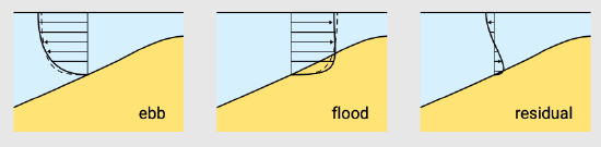
The combination of suspended load transport with secondary flows can give a net sediment transport, even though the depth-averaged velocity is zero. This is the result of the non-uniform distribution of the sediment concentration over the vertical: most of the sediment is concentrated in the lower part of the water column. An example is the above discussed cross-shore secondary flow under breaking waves that gives a net transport component against the direction of wave propagation; the sediment concentrations are largest in the lower layers of the water column, where the velocity is offshore directed (undertow). Under non-breaking waves, wave-induced streaming close to the bed may result in an onshore directed transport. In the same way, secondary flows in a tidal basin can have a net effect on the transport direction. The curvature-induced secondary flow in a channel bend (Sect. 5.7.6), for instance, will give a net transport component towards the centre of curvature (from the outer bend to the inner bend). Another potentially important contribution of this type is associated with the deformation of the velocity profile as the flow moves up or down a steep slope (see Fig. 6.15). When averaged over the tide, this gives a net upslope transport. This may explain why steep banks of tidal channels can be stable.