5.7.5: Overtides

Last updated
Save as PDF

Page ID: 16339

Judith Bosboom & Marcel J.F. Stive
Delft University of Technology via TU Delft Open

\( \newcommand{\vecs}[1]{\overset { \scriptstyle \rightharpoonup} {\mathbf{#1}} } \) \( \newcommand{\vecd}[1]{\overset{-\!-\!\rightharpoonup}{\vphantom{a}\smash {#1}}} \)\(\newcommand{\id}{\mathrm{id}}\) \( \newcommand{\Span}{\mathrm{span}}\) \( \newcommand{\kernel}{\mathrm{null}\,}\) \( \newcommand{\range}{\mathrm{range}\,}\) \( \newcommand{\RealPart}{\mathrm{Re}}\) \( \newcommand{\ImaginaryPart}{\mathrm{Im}}\) \( \newcommand{\Argument}{\mathrm{Arg}}\) \( \newcommand{\norm}[1]{\| #1 \|}\) \( \newcommand{\inner}[2]{\langle #1, #2 \rangle}\) \( \newcommand{\Span}{\mathrm{span}}\) \(\newcommand{\id}{\mathrm{id}}\) \( \newcommand{\Span}{\mathrm{span}}\) \( \newcommand{\kernel}{\mathrm{null}\,}\) \( \newcommand{\range}{\mathrm{range}\,}\) \( \newcommand{\RealPart}{\mathrm{Re}}\) \( \newcommand{\ImaginaryPart}{\mathrm{Im}}\) \( \newcommand{\Argument}{\mathrm{Arg}}\) \( \newcommand{\norm}[1]{\| #1 \|}\) \( \newcommand{\inner}[2]{\langle #1, #2 \rangle}\) \( \newcommand{\Span}{\mathrm{span}}\)\(\newcommand{\AA}{\unicode[.8,0]{x212B}}\)

Mathematically, tidal distortion and asymmetry can be described by the inclusion of higher harmonics, tidal periods that do not originate from a tidal forcing period but are integer fractions (1/2, 1/3, etc.) of the period of the basic astronomical constituents generated by the attraction forces of earth, moon and sun. For that reason they are named overtides. Since these higher harmonics are generated as a result of non-linear effects in shallowing coastal waters and tidal basins (compare with wind waves, Sect. 5.5), they are also called shallow-water tides. The phase relationships between the tidal constituents determine whether the tidal elevation and velocity curves are asymmetric about the horizontal or about the vertical axis.

Two important sources for non-linearity in the tidal propagation equations are bottom friction and continuity. The continuity equation Eq. 5.7.3.2 or Eq. 5.7.3.1 leads to \(c = \sqrt{gh}\) or \(c = \sqrt{gA_s/b}\). Different celerities of the high and low tide were seen to introduce tidal asymmetry. The resulting distortion of the surface elevation profile can be approxim- ated with a second harmonic: a wave with twice the frequency of the basic harmonic. Equivalently, non-linear tidal propagation in shallow water thus generates a M4 tide from the M2 tide with a period that is 1/2 the M2 period. In the same way additional higher harmonics can be generated (M8, etc.). The higher harmonics to S2 are S4, S8, etc. If the different tidal components interact, interaction tides can be generated, e.g., M2 and S2 can generate MS4 (see Table 3.6). This explains why Table 3.6 is so much longer than Table 3.5!

The second source of higher harmonics is the quadratic (and hence non-linear) bottom friction term \(\tau_b = \rho c_f u|u| \propto \cos \omega t |\cos \omega t|\). A Fourier expansion of this term can be shown to give tidal constituents with a frequency that is three times as high as the basic frequency. Friction thus generates a M6 tide from the M2 tide with a period that is 1/3 of the M2 period. Similarly, from S2 the S6 tide is generated. In the denominator of the friction term in Eq. 5.7.3.4 we have the water depth \(h\), which varies with the tidal stage. This will introduce second harmonics (M4 etc.).

截屏2021-10-25 下午10.52.56.png — Figure 5.71: Influence of the relative phase difference between the M2 and M4 tide on the asymmetry about the horizontal axis and vertical axis. The combined signal becomes positively skewed when the two are in phase (left panel), asymmetric (w.r.t. the vertical axis, i.e., leaning forward in space, hence backward in time) when the phase shift \(\varphi_{M4} - 2\varphi_{M2} = -\pi /2\) (middle panel), and negatively skewed when the two are out of phase (i.e., \(\varphi_{M4} - 2\varphi_{M2} = \pm \pi\), right panel). Note that not depicted is \(\varphi_{M2} - 2\varphi_{M2} = \pi /2\) which would result in a backward leaning signal in space and forward leaning signal in time.

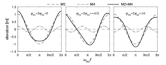
Figure 5.71 demonstrates the effect of the summation of M2 (semidiurnal, \(12.42\ h\) period) and M4 (quarter-diurnal, \(6.21\ h\) period) with amplitudes of \(a_{M4} = 1\ m\) and \(a_{M2} = 0.2\ m\) respectively. The surface elevation is given by:

\[\eta (t) = a_{M2} \cos (\omega_{M2} t - \varphi_{M2}) + a_{M4} \cos (\omega_{M4} t - \varphi_{M4})\]

Since \(\omega_{M4} = 2\omega_{M2}\) and with \(t' = t - \varphi_{M2}/\omega_{M2}\), this can be written as:

\[\eta (t) = a_{M2} \cos (\omega_{M2} t') + a_{M4} \cos (2\omega_{M2} t' - (\varphi_{M4} - 2 \varphi_{M2}))\]

On the \(x\)-axis of Figure 5.71 we have \(\omega_{M2} t'\) in degrees. The phase lag between M2 and M4 is \(\varphi_{M4} - 2\varphi_{M2}\). If the phase lag is \(0^{\circ}\) or \(\pm 180^{\circ}\) the result is an asymmetry about the horizontal (either a positive or negative skewness). For \(\varphi_{M4} - 2\varphi_{M2} = 0^{\circ}\) the signal is positively skewed (left panel), for \(\varphi_{M4} - 2\varphi_{M2} = \pm 180^{\circ}\) it is negatively skewed (right panel). If \(\varphi_{M4} - 2\varphi_{M2} = \pm 90^{\circ}\) the result is an asymmetry about the vertical axis (a longer falling period than rising period or vice versa). Shown in the figure is the situation that the falling period is longer than the rising period (middle panel). For relative phase differences other than the special cases of \(0^{\circ}\), \(\pm 90^{\circ}\) and \(\pm 180^{\circ}\), the two types of asymmetry will be combined.

Sediment transport as a result of asymmetry of the horizontal tide is explained in Sect. 9.7 in terms of the overtides.