3.9: Tidal analysis and prediction

Last updated
Save as PDF

Page ID: 16309

Judith Bosboom & Marcel J.F. Stive
Delft University of Technology via TU Delft Open

\( \newcommand{\vecs}[1]{\overset { \scriptstyle \rightharpoonup} {\mathbf{#1}} } \) \( \newcommand{\vecd}[1]{\overset{-\!-\!\rightharpoonup}{\vphantom{a}\smash {#1}}} \)\(\newcommand{\id}{\mathrm{id}}\) \( \newcommand{\Span}{\mathrm{span}}\) \( \newcommand{\kernel}{\mathrm{null}\,}\) \( \newcommand{\range}{\mathrm{range}\,}\) \( \newcommand{\RealPart}{\mathrm{Re}}\) \( \newcommand{\ImaginaryPart}{\mathrm{Im}}\) \( \newcommand{\Argument}{\mathrm{Arg}}\) \( \newcommand{\norm}[1]{\| #1 \|}\) \( \newcommand{\inner}[2]{\langle #1, #2 \rangle}\) \( \newcommand{\Span}{\mathrm{span}}\) \(\newcommand{\id}{\mathrm{id}}\) \( \newcommand{\Span}{\mathrm{span}}\) \( \newcommand{\kernel}{\mathrm{null}\,}\) \( \newcommand{\range}{\mathrm{range}\,}\) \( \newcommand{\RealPart}{\mathrm{Re}}\) \( \newcommand{\ImaginaryPart}{\mathrm{Im}}\) \( \newcommand{\Argument}{\mathrm{Arg}}\) \( \newcommand{\norm}[1]{\| #1 \|}\) \( \newcommand{\inner}[2]{\langle #1, #2 \rangle}\) \( \newcommand{\Span}{\mathrm{span}}\)\(\newcommand{\AA}{\unicode[.8,0]{x212B}}\)

Because the tide is caused by regular astronomical phenomena, it can be predicted accurately a long time ahead (although not including meteorological effects as storm surges). The method used for tide prediction is harmonic analysis. Analogous to the treatment of wind waves, the water level at a certain location as a function of time is expressed by the following formula:

\[\eta (t) = a_0 + \sum_{n = 1}^{N} a_n \cos (\omega_n t - \alpha_n)\label{eq3.9.1}\]

where

\(\eta_t\)	measured (or predicted) tidal level with reference to a fiexed level	\(m\)
\(a_0\)	mean level	\(m\)
\(a_n\)	amplitude of component number \(n\)	\(m\)
\(\omega_n\)	angular velocity of component number \(n\)	\(1/h\)
\(a_n\)	phase angle of component number \(n\)	-
\(t\)	time	\(h\)
\(N\)	number of harmonic components	-

Contrary to the traditional harmonic analysis, the frequencies \(\omega_n\) are known here, having been derived from astronomical considerations. The phase angles \(\alpha_n\) have to be derived from observations as they are extremely site specific. This applies to the amplitudes \(a_n\) as well. Tidal analysis for a certain location therefore is the determination of amplitudes and phases. Note that the phase angles are a function of the adopted time-origin.

The length of the analysed water level record determines the number of constituents that can be determined. A year’s length can unravel the main constituents, except for the constituent with the period of 18.6 yr. The effect of this can be introduced by adjusting amplitudes and phases according to the position in that long-term cycle. Instead of Eq. \(\ref{eq3.9.1}\) we then get:

\[\eta (t) = a_0 + \sum_{n = 1}^{N} f_n a_n \cos (\omega_n t - \alpha_n + \beta_n)\]

Here \(f_n\) is the so-called nodal factor that captures the effect of the 18.6 yr cycle on the tidal amplitudes. The correction to the phase is given by \(\beta_n\). The nodal modulation can also be used to reduce the number of constituents in a tidal analysis; since the tidal constituents are gathered in groups with similar frequencies (see Fig. 3.27), the effect of smaller amplitude constituents in a group can be taken into account via corrections to the amplitude and phase of the main, larger amplitude constituent in the group.

When the tidal constituents are known for a certain location, they can be used to predict future tides. For many ports in the world the tidal constituents are known and published and can be used. If for a project local tidal constituents are not known, two solutions can be chosen. The first is to collect local data with a short period (for instance a month) from which the most important constituents can be determined. Another possibility is to use data from a nearby station and use a model for tidal propagation to determine the amplitudes and phases for the project site.

An example of the result of a harmonic analysis for some ports along the Dutch coast is presented in Table 3.6. This table shows the main harmonic components used for prediction of the astronomic tide. Each component has an internationally agreed abbreviation. The most important constituents have already been discussed in Sect. 3.7.6. Besides those principal constituents, each constituent may also have higher harmonics, generated by non-linearities. Higher order components carry a subscript 3, 4 or higher. From the table one can see that the ratio of the effects of the sun and the moon is approximately 1 to 4 along the Dutch coast (ratio \(S2/M2 \approx 1/4\)).

截屏2021-10-18 下午9.31.07.png

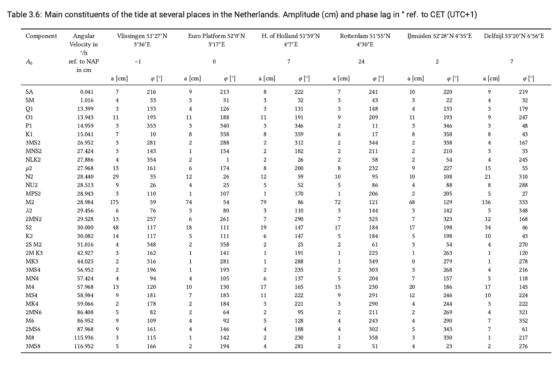
Nota bene: in Table 3.6, the mean level is denoted by \(A_0\) and gives the mean difference between Normaal Amsterdams Peil in Dutch (NAP) (fixed reference level) and MSL. MSL is the mean level as determined from measurements and is the level without tides and averaged meteorological effects. Close to the coast this difference can be neglected; but if one looks at a river farther upstream, the river gradient influences the mean sea level. The difference between NAP and MSL changes a little during the year, as can be seen from the small amplitude of component SA. The angular velocity of this component (0.041) leads to a period of 365 d.

Contrary to the Dutch tide tables, in other such tables \(A_0\) represents the difference between a Chart Datum and MSL. Chart Datum is then defined as a low level that is exceeded rarely, for instance Lowest Astronomical Tide (LAT) or Mean Lower Low Water (MLLW). LAT is defined as the lowest tide level which can be predicted to occur under average meteorological conditions and under any combination of astronomical conditions. MLLW is the average height of the lower of the two daily low waters over a long period of time. When only one low water occurs on a day, this is taken as the lower low water.

Because of this site-specific definition of the Datum level, the Datum plane is not necessarily horizontal. Utmost care is required when performing hydraulic calculations in this case (see also App. C). The Datum level used by different countries for the same waterway can also be different, which leads to different depth figures for the same location. This is the case for the Western Scheldt, where Dutch and Belgian charts show such differences.

Tidal levels like MLLW are long-term averaged tidal levels based on measurements and therefore include averaged meteorological influences on the water level. The period of averaging is preferably 18.6 years, so that tidal component with this duration is properly taken into account. Commonly used long-term averaged tidal levels are for instance Mean Low Water (MLW) and Mean High Water (MHW). Other tidal levels are defined in App. C.

The tidal range can be defined using different tidal levels. The normal tidal range is defined as MHW – MLW. But also the spring tidal range (Mean High Water Spring (MHWS) – Mean Low Water Spring (MLWS)) or neap tidal range (Mean High Water Neap (MHWN) – Mean Low Water Neap (MLWN)) can be used.

In morphodynamic modelling preferably a complete spring-neap tide cycle is taken into account. This is however computationally demanding. To reduce computational costs, a so-called morphological representative tide can be used. This is a single tidal cycle that is expected to have a similar effect on the morphology as the total spring-neap tidal cycle.