3.7.6: Tidal constituents

The principal tidal constituents are shown in Table 3.5. We have seen in Sect. 3.7.3 that the main lunar tide has a period of 12.42 h and the main solar tide a period of 12 h respectively. These tidal constituents (or tidal components) are called \(M2\) and \(S2\). The influence of the sun is characterised by the letter \(S\), the influence of the moon by the letter \(M\). The index 2 refers to phenomena that occur twice daily. The amplitudes and phases of these two constituents vary with the location at the earth.

Table 3.5: Principal tidal constituents with equilibrium amplitudes from Apel (1987)

Tidal constituents	Name	Equilibrium Amplitude [m]	Period [h]
Semidiurnal
Principal lunar	M2	0.24	12.42
Principal solar	S2	0.11	12.00
Lunar elliptical	N2	0.046	12.66
Lunar-solar declinational	K2	0.031	11.97
Diurnal
Lunar-solar declinational	K1	0.14	23.93
Principal lunar	O1	0.10	25.82
Principal solar	P1	0.047	24.07
Lunar elliptical	Q1	0.019	26.87
Long Period
Fortnightly	Mf	0.042	327.9
Monthly	Mm	0.022	661.3
Semiannual	Ssa	0.019	4383

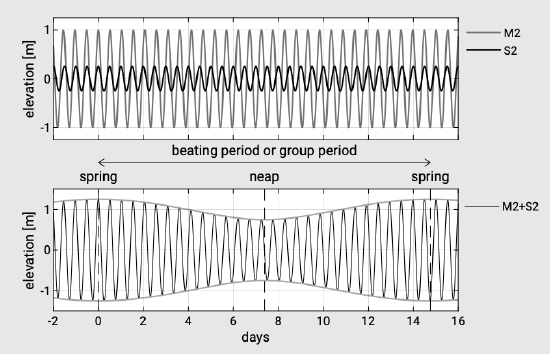
The tidal variations are in the order of decimetres only in the open oceans. According to equilibrium theory the amplitudes of \(M2\) and \(S2\) are 0.24 m and 0.11 m respectively. This gives a ratio of \(S2/M2\) = 0.46 which could also be calculated using Eqs. 3.7.3.1 and 3.7.3.2 as \(S2/M2\) = 0.515/1.13 = 0.46. The \(M2\) and \(S2\) signals have a slightly different frequency resulting in a so-called beating of the two signals resulting in spring-neap tide variability: when the \(M2\) and \(S2\) components are in phase (the moon and the sun are aligned) it is spring tide and when they are out of phase it is neap tide. This we had seen before in Sect. 3.7.4. The beating of the two signals resulting in a variation of the amplitudes over the lunar month is comparable to the beating of two wave trains with slightly different frequencies resulting in amplitude variation or modulation on a wave group scale as treated in Sect. 3.5.3. Intermezzo 3.4 treats this amplitude modulation in more detail.

Intermezzo 3.4 Astronomical constituents

Figure 3.25: The interaction between \(M2\) and \(S2\) results in a spring and neap tide variation. Verify that the beating period of \(M2\) and \(S2\) is 14.7 days (cf. the group period for wind waves Eq. 3.5.3.2).

Section 3.7.6 described the ocean tide as a sinusoidal semi-diurnal water level vari- ation modified with a fortnightly spring and neap tide variation and with a daily inequality. The spring and neap tide variation is the result of the linear summation of principal components with a small differential frequency. Consider the \(M2\) and \(S2\) components. The linear combination of these two tidal components with a small difference in frequency results in an amplitude variation with a period determined by \(\omega_{S2} - \omega_{M2}\), comparable to the beating of two short wave trains with slightly different frequencies (see Sect. 3.5.3). This is shown in Fig. 3.25.

Figure 3.26: The interaction between \(M2\) and \(K1\) leads to a daily inequality between two successive high waters and between two successive low waters. Also, a slower amplitude variation can be observed.

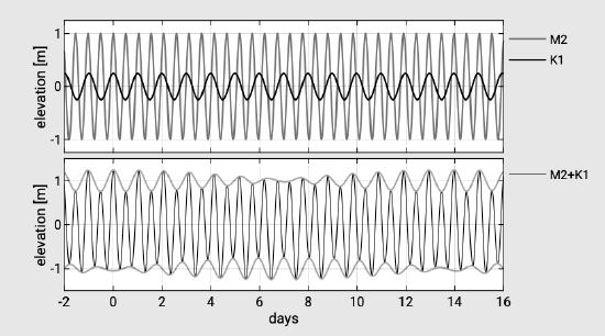
The daily inequality for a predominantly semi-diurnal tide is the result of the summation of a semi-diurnal and a diurnal component and is demonstrated in Fig. 3.26 for \(M2\) and \(K1\). The result is the succession of two symmetrical tides with different tidal range (the difference between the elevations of the two successive high waters is called daily inequality).

The declination of the earth axis introduces semi-diurnal and diurnal tidal constituents \(K1\), \(K2\) and \(O1\) and \(P1\). Diurnal components carry a subscript 1. \(K1\) with \(O1\) expresses the effect of the moon’s declination, \(K1\) with \(P1\) of the sun’s declination. \(K1\), \(P1\) and \(O1\) account for diurnal inequality (see Intermezzo 3.4) and, at extremes, diurnal tides (where the semi-diurnal component has disappeared completely). The \(K2\) constituent modulates the amplitude and frequency of \(M2\) and \(S2\) for the declinational effect of the moon and the sun, respectively. Other effects will generate other tidal constituents defined by an exact period, with their own amplitudes according to equilibrium theory and with their own phases with respect to each other. For instance, the moon’s distance from the earth varies because the moon’s orbit is elliptical and because the elliptical orbit is not fixed. This effect introduces semi-diurnal and diurnal constituents \(N2\) and \(Q1\). The longest period is 18.6 years which is the period of the 5° variation of the lunar declination.

For practical purposes, the tide can be seen as a sinusoidal semi-diurnal water level variation modified with a fortnightly spring and neap tide amplitude variation and with a daily inequality that varies with latitude and with the monthly and annual cycle. In the extreme case the daily inequality is so large that the water level variation is solely diurnal.

Figure 3.27: Spectrum of equilibrium tides with frequencies near twice per day. Upper: the spectrum is split into groups separated by a cycle per month (0.55 °/h). Lower: expanded spectrum of the \(S2\) group, showing splitting at a cycle per year (0.04 °/h). The finest splitting in this figure is at a cycle per 8.847 years (0.0046 °/h). (From Richard Eanes, Center for Space Research, University of Texas in Stewart, 2008, see also https://github.com/introocean/introocean-en).

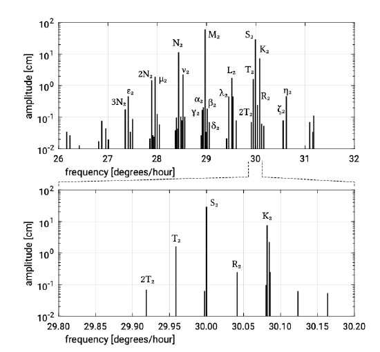
\(M2\) and \(S2\) are the main but not the only constituents with frequencies near twice per day (see Fig. 3.27). Note that the spectrum of equilibrium tides in Fig. 3.27 consists of discrete lines; tides have precise frequencies determined by the orbits of the earth and moon, and their spectrum is not continuous. We have seen before that ocean waves have all possible frequencies, and their spectrum is continuous.