
20: Numerical Weather Prediction (NWP)
- Page ID
- 9665

\( \newcommand{\vecs}[1]{\overset { \scriptstyle \rightharpoonup} {\mathbf{#1}} } \)
\( \newcommand{\vecd}[1]{\overset{-\!-\!\rightharpoonup}{\vphantom{a}\smash {#1}}} \)
\( \newcommand{\dsum}{\displaystyle\sum\limits} \)
\( \newcommand{\dint}{\displaystyle\int\limits} \)
\( \newcommand{\dlim}{\displaystyle\lim\limits} \)
\( \newcommand{\id}{\mathrm{id}}\) \( \newcommand{\Span}{\mathrm{span}}\)
( \newcommand{\kernel}{\mathrm{null}\,}\) \( \newcommand{\range}{\mathrm{range}\,}\)
\( \newcommand{\RealPart}{\mathrm{Re}}\) \( \newcommand{\ImaginaryPart}{\mathrm{Im}}\)
\( \newcommand{\Argument}{\mathrm{Arg}}\) \( \newcommand{\norm}[1]{\| #1 \|}\)
\( \newcommand{\inner}[2]{\langle #1, #2 \rangle}\)
\( \newcommand{\Span}{\mathrm{span}}\)
\( \newcommand{\id}{\mathrm{id}}\)
\( \newcommand{\Span}{\mathrm{span}}\)
\( \newcommand{\kernel}{\mathrm{null}\,}\)
\( \newcommand{\range}{\mathrm{range}\,}\)
\( \newcommand{\RealPart}{\mathrm{Re}}\)
\( \newcommand{\ImaginaryPart}{\mathrm{Im}}\)
\( \newcommand{\Argument}{\mathrm{Arg}}\)
\( \newcommand{\norm}[1]{\| #1 \|}\)
\( \newcommand{\inner}[2]{\langle #1, #2 \rangle}\)
\( \newcommand{\Span}{\mathrm{span}}\) \( \newcommand{\AA}{\unicode[.8,0]{x212B}}\)
\( \newcommand{\vectorA}[1]{\vec{#1}} % arrow\)
\( \newcommand{\vectorAt}[1]{\vec{\text{#1}}} % arrow\)
\( \newcommand{\vectorB}[1]{\overset { \scriptstyle \rightharpoonup} {\mathbf{#1}} } \)
\( \newcommand{\vectorC}[1]{\textbf{#1}} \)
\( \newcommand{\vectorD}[1]{\overrightarrow{#1}} \)
\( \newcommand{\vectorDt}[1]{\overrightarrow{\text{#1}}} \)
\( \newcommand{\vectE}[1]{\overset{-\!-\!\rightharpoonup}{\vphantom{a}\smash{\mathbf {#1}}}} \)
\( \newcommand{\vecs}[1]{\overset { \scriptstyle \rightharpoonup} {\mathbf{#1}} } \)
\(\newcommand{\longvect}{\overrightarrow}\)
\( \newcommand{\vecd}[1]{\overset{-\!-\!\rightharpoonup}{\vphantom{a}\smash {#1}}} \)
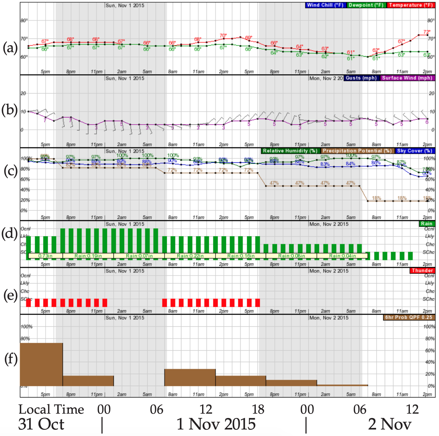
\(\newcommand{\avec}{\mathbf a}\) \(\newcommand{\bvec}{\mathbf b}\) \(\newcommand{\cvec}{\mathbf c}\) \(\newcommand{\dvec}{\mathbf d}\) \(\newcommand{\dtil}{\widetilde{\mathbf d}}\) \(\newcommand{\evec}{\mathbf e}\) \(\newcommand{\fvec}{\mathbf f}\) \(\newcommand{\nvec}{\mathbf n}\) \(\newcommand{\pvec}{\mathbf p}\) \(\newcommand{\qvec}{\mathbf q}\) \(\newcommand{\svec}{\mathbf s}\) \(\newcommand{\tvec}{\mathbf t}\) \(\newcommand{\uvec}{\mathbf u}\) \(\newcommand{\vvec}{\mathbf v}\) \(\newcommand{\wvec}{\mathbf w}\) \(\newcommand{\xvec}{\mathbf x}\) \(\newcommand{\yvec}{\mathbf y}\) \(\newcommand{\zvec}{\mathbf z}\) \(\newcommand{\rvec}{\mathbf r}\) \(\newcommand{\mvec}{\mathbf m}\) \(\newcommand{\zerovec}{\mathbf 0}\) \(\newcommand{\onevec}{\mathbf 1}\) \(\newcommand{\real}{\mathbb R}\) \(\newcommand{\twovec}[2]{\left[\begin{array}{r}#1 \\ #2 \end{array}\right]}\) \(\newcommand{\ctwovec}[2]{\left[\begin{array}{c}#1 \\ #2 \end{array}\right]}\) \(\newcommand{\threevec}[3]{\left[\begin{array}{r}#1 \\ #2 \\ #3 \end{array}\right]}\) \(\newcommand{\cthreevec}[3]{\left[\begin{array}{c}#1 \\ #2 \\ #3 \end{array}\right]}\) \(\newcommand{\fourvec}[4]{\left[\begin{array}{r}#1 \\ #2 \\ #3 \\ #4 \end{array}\right]}\) \(\newcommand{\cfourvec}[4]{\left[\begin{array}{c}#1 \\ #2 \\ #3 \\ #4 \end{array}\right]}\) \(\newcommand{\fivevec}[5]{\left[\begin{array}{r}#1 \\ #2 \\ #3 \\ #4 \\ #5 \\ \end{array}\right]}\) \(\newcommand{\cfivevec}[5]{\left[\begin{array}{c}#1 \\ #2 \\ #3 \\ #4 \\ #5 \\ \end{array}\right]}\) \(\newcommand{\mattwo}[4]{\left[\begin{array}{rr}#1 \amp #2 \\ #3 \amp #4 \\ \end{array}\right]}\) \(\newcommand{\laspan}[1]{\text{Span}\{#1\}}\) \(\newcommand{\bcal}{\cal B}\) \(\newcommand{\ccal}{\cal C}\) \(\newcommand{\scal}{\cal S}\) \(\newcommand{\wcal}{\cal W}\) \(\newcommand{\ecal}{\cal E}\) \(\newcommand{\coords}[2]{\left\{#1\right\}_{#2}}\) \(\newcommand{\gray}[1]{\color{gray}{#1}}\) \(\newcommand{\lgray}[1]{\color{lightgray}{#1}}\) \(\newcommand{\rank}{\operatorname{rank}}\) \(\newcommand{\row}{\text{Row}}\) \(\newcommand{\col}{\text{Col}}\) \(\renewcommand{\row}{\text{Row}}\) \(\newcommand{\nul}{\text{Nul}}\) \(\newcommand{\var}{\text{Var}}\) \(\newcommand{\corr}{\text{corr}}\) \(\newcommand{\len}[1]{\left|#1\right|}\) \(\newcommand{\bbar}{\overline{\bvec}}\) \(\newcommand{\bhat}{\widehat{\bvec}}\) \(\newcommand{\bperp}{\bvec^\perp}\) \(\newcommand{\xhat}{\widehat{\xvec}}\) \(\newcommand{\vhat}{\widehat{\vvec}}\) \(\newcommand{\uhat}{\widehat{\uvec}}\) \(\newcommand{\what}{\widehat{\wvec}}\) \(\newcommand{\Sighat}{\widehat{\Sigma}}\) \(\newcommand{\lt}{<}\) \(\newcommand{\gt}{>}\) \(\newcommand{\amp}{&}\) \(\definecolor{fillinmathshade}{gray}{0.9}\)Most weather forecasts are made by computer, and some of these forecasts are further enhanced by humans. Computers can keep track of myriad complex nonlinear interactions among winds, temperature, and moisture at thousands of locations and altitudes around the world — an impossible task for humans. Also, data observation, collection, analysis, display and dissemination are mostly automated.
Fig. 20.1 shows an automated forecast. Produced by computer, this meteogram (graph of weather vs. time for one location) is easier for non-meteorologists to interpret than weather maps. But to produce such forecasts, the equations describing the atmosphere must first be solved.
- 20.1: Scientific Basis of Forecasting
- This page covers essential concepts in numerical weather forecasting, focusing on the equations of motion like the Eulerian equations for atmospheric variables, and discusses heat and moisture conservation. It highlights the transformation of coordinates for modeling, particularly map projections and their importance.
- 20.2: Grid Points
- This page discusses Moore's Law, which indicates that transistor density on integrated circuits doubles approximately every two years, leading to greater computing power. This advancement improves numerical weather prediction (NWP) models, allowing for finer grid resolutions but also raising computational requirements. Techniques such as nested and variable grids, as well as staggered grid layouts, enhance forecasting accuracy and efficiency by addressing challenges in simpler grid structures.
- 20.3: Finite-Difference Equations
- This page explores various numerical methods for approximating equations of motion in weather prediction. Key topics include discrete approximations for spatial gradients, using Taylor series and finite difference methods to enhance accuracy. It highlights the significance of truncation techniques, grid point calculations, and the leapfrog time-differencing scheme for stability and forecasting.
- 20.4: Numerical Errors and Instability
- This page covers the sources of errors in Numerical Weather Prediction (NWP), including round-off, truncation, and numerical instabilities, and traces the historical development of NWP. It also details the design considerations for a hurricane forecasting model, emphasizing the necessary grid and domain sizes, along with computational requirements.
- 20.5: The Numerical Forecast Process
- This page outlines the integral role of mathematical models and data assimilation techniques in weather forecasting, emphasizing the phases of data processing and the importance of accurate initial conditions. It discusses how initialization errors can adversely affect forecasts, particularly in data-sparse regions. Two main data assimilation methods—optimum interpolation and variational data assimilation—are highlighted for optimizing initial conditions.
- 20.6: Nonlinear Dynamics and Chaos
- This page explores Ed Lorenz's significant contributions to chaos theory and its implications for weather forecasting, specifically highlighting sensitive dependence on initial conditions. It discusses the inadequacy of traditional forecasting methods and introduces ensemble forecasts that use varied initial conditions to capture uncertainty.
- 20.7: Forecast Quality and Verfication
- This page covers various methods and metrics for evaluating weather forecasts, including systematic and random errors in Numerical Weather Prediction (NWP). It details the use of ensemble forecasting, Model Output Statistics, and verification metrics such as mean errors and correlation coefficients. Additionally, it discusses binary forecasting, contingency tables, Brier Skill Scores, and Receiver Operating Characteristic (ROC) curves to assess forecast reliability.
- 20.8. Review
- This page discusses the atmosphere's role in weather forecasting, emphasizing fluid mechanics and thermodynamics. It highlights the complexity of governing equations and the reliance on finite-difference approximations with grid cells. Initial conditions are updated with observations, but parameterization is necessary due to resolution limits. Various errors can affect forecasts, leading to systematic biases.
- 20.9: Homework Exercises
- This page covers operational weather forecasting tasks, focusing on numerical weather prediction (NWP) models and meteorological data. It examines major weather forecast centers, model validation with observational data, and historical advancements in forecasting. Key topics include the impact of observational data on accuracy, the benefits of computational advancements, model grid arrangements, and predictability limits.