20.5: The Numerical Forecast Process
- Page ID
- 9663
\( \newcommand{\vecs}[1]{\overset { \scriptstyle \rightharpoonup} {\mathbf{#1}} } \)
\( \newcommand{\vecd}[1]{\overset{-\!-\!\rightharpoonup}{\vphantom{a}\smash {#1}}} \)
\( \newcommand{\id}{\mathrm{id}}\) \( \newcommand{\Span}{\mathrm{span}}\)
( \newcommand{\kernel}{\mathrm{null}\,}\) \( \newcommand{\range}{\mathrm{range}\,}\)
\( \newcommand{\RealPart}{\mathrm{Re}}\) \( \newcommand{\ImaginaryPart}{\mathrm{Im}}\)
\( \newcommand{\Argument}{\mathrm{Arg}}\) \( \newcommand{\norm}[1]{\| #1 \|}\)
\( \newcommand{\inner}[2]{\langle #1, #2 \rangle}\)
\( \newcommand{\Span}{\mathrm{span}}\)
\( \newcommand{\id}{\mathrm{id}}\)
\( \newcommand{\Span}{\mathrm{span}}\)
\( \newcommand{\kernel}{\mathrm{null}\,}\)
\( \newcommand{\range}{\mathrm{range}\,}\)
\( \newcommand{\RealPart}{\mathrm{Re}}\)
\( \newcommand{\ImaginaryPart}{\mathrm{Im}}\)
\( \newcommand{\Argument}{\mathrm{Arg}}\)
\( \newcommand{\norm}[1]{\| #1 \|}\)
\( \newcommand{\inner}[2]{\langle #1, #2 \rangle}\)
\( \newcommand{\Span}{\mathrm{span}}\) \( \newcommand{\AA}{\unicode[.8,0]{x212B}}\)
\( \newcommand{\vectorA}[1]{\vec{#1}} % arrow\)
\( \newcommand{\vectorAt}[1]{\vec{\text{#1}}} % arrow\)
\( \newcommand{\vectorB}[1]{\overset { \scriptstyle \rightharpoonup} {\mathbf{#1}} } \)
\( \newcommand{\vectorC}[1]{\textbf{#1}} \)
\( \newcommand{\vectorD}[1]{\overrightarrow{#1}} \)
\( \newcommand{\vectorDt}[1]{\overrightarrow{\text{#1}}} \)
\( \newcommand{\vectE}[1]{\overset{-\!-\!\rightharpoonup}{\vphantom{a}\smash{\mathbf {#1}}}} \)
\( \newcommand{\vecs}[1]{\overset { \scriptstyle \rightharpoonup} {\mathbf{#1}} } \)
\( \newcommand{\vecd}[1]{\overset{-\!-\!\rightharpoonup}{\vphantom{a}\smash {#1}}} \)
\(\newcommand{\avec}{\mathbf a}\) \(\newcommand{\bvec}{\mathbf b}\) \(\newcommand{\cvec}{\mathbf c}\) \(\newcommand{\dvec}{\mathbf d}\) \(\newcommand{\dtil}{\widetilde{\mathbf d}}\) \(\newcommand{\evec}{\mathbf e}\) \(\newcommand{\fvec}{\mathbf f}\) \(\newcommand{\nvec}{\mathbf n}\) \(\newcommand{\pvec}{\mathbf p}\) \(\newcommand{\qvec}{\mathbf q}\) \(\newcommand{\svec}{\mathbf s}\) \(\newcommand{\tvec}{\mathbf t}\) \(\newcommand{\uvec}{\mathbf u}\) \(\newcommand{\vvec}{\mathbf v}\) \(\newcommand{\wvec}{\mathbf w}\) \(\newcommand{\xvec}{\mathbf x}\) \(\newcommand{\yvec}{\mathbf y}\) \(\newcommand{\zvec}{\mathbf z}\) \(\newcommand{\rvec}{\mathbf r}\) \(\newcommand{\mvec}{\mathbf m}\) \(\newcommand{\zerovec}{\mathbf 0}\) \(\newcommand{\onevec}{\mathbf 1}\) \(\newcommand{\real}{\mathbb R}\) \(\newcommand{\twovec}[2]{\left[\begin{array}{r}#1 \\ #2 \end{array}\right]}\) \(\newcommand{\ctwovec}[2]{\left[\begin{array}{c}#1 \\ #2 \end{array}\right]}\) \(\newcommand{\threevec}[3]{\left[\begin{array}{r}#1 \\ #2 \\ #3 \end{array}\right]}\) \(\newcommand{\cthreevec}[3]{\left[\begin{array}{c}#1 \\ #2 \\ #3 \end{array}\right]}\) \(\newcommand{\fourvec}[4]{\left[\begin{array}{r}#1 \\ #2 \\ #3 \\ #4 \end{array}\right]}\) \(\newcommand{\cfourvec}[4]{\left[\begin{array}{c}#1 \\ #2 \\ #3 \\ #4 \end{array}\right]}\) \(\newcommand{\fivevec}[5]{\left[\begin{array}{r}#1 \\ #2 \\ #3 \\ #4 \\ #5 \\ \end{array}\right]}\) \(\newcommand{\cfivevec}[5]{\left[\begin{array}{c}#1 \\ #2 \\ #3 \\ #4 \\ #5 \\ \end{array}\right]}\) \(\newcommand{\mattwo}[4]{\left[\begin{array}{rr}#1 \amp #2 \\ #3 \amp #4 \\ \end{array}\right]}\) \(\newcommand{\laspan}[1]{\text{Span}\{#1\}}\) \(\newcommand{\bcal}{\cal B}\) \(\newcommand{\ccal}{\cal C}\) \(\newcommand{\scal}{\cal S}\) \(\newcommand{\wcal}{\cal W}\) \(\newcommand{\ecal}{\cal E}\) \(\newcommand{\coords}[2]{\left\{#1\right\}_{#2}}\) \(\newcommand{\gray}[1]{\color{gray}{#1}}\) \(\newcommand{\lgray}[1]{\color{lightgray}{#1}}\) \(\newcommand{\rank}{\operatorname{rank}}\) \(\newcommand{\row}{\text{Row}}\) \(\newcommand{\col}{\text{Col}}\) \(\renewcommand{\row}{\text{Row}}\) \(\newcommand{\nul}{\text{Nul}}\) \(\newcommand{\var}{\text{Var}}\) \(\newcommand{\corr}{\text{corr}}\) \(\newcommand{\len}[1]{\left|#1\right|}\) \(\newcommand{\bbar}{\overline{\bvec}}\) \(\newcommand{\bhat}{\widehat{\bvec}}\) \(\newcommand{\bperp}{\bvec^\perp}\) \(\newcommand{\xhat}{\widehat{\xvec}}\) \(\newcommand{\vhat}{\widehat{\vvec}}\) \(\newcommand{\uhat}{\widehat{\uvec}}\) \(\newcommand{\what}{\widehat{\wvec}}\) \(\newcommand{\Sighat}{\widehat{\Sigma}}\) \(\newcommand{\lt}{<}\) \(\newcommand{\gt}{>}\) \(\newcommand{\amp}{&}\) \(\definecolor{fillinmathshade}{gray}{0.9}\)“To have to translate one’s verbal statement into mathematical formulae compels one to scrutinize the ideas therein expressed. Next the possession of formulae makes it much easier to deduce the consequences. In this way absurd implications, which might have passed unnoticed in a verbal statement, are brought clearly into view & stimulate one to amend the formula.
Mathematical expressions have, however, their special tendencies to pervert thought: the definiteness may be spurious, existing in the equation but not in the phenomena to be described; and the brevity may be due to the omission of the more important things, simply because they cannot be mathematized. Against these faults we must constantly be on our guard.”
– L.F. Richardson, 1919
Weather forecasting is an initial value problem. As shown in eq. (20.17), you must know the initial conditions on the right hand side in order to forecast the temperature at later times (t + ∆t). Thus, to make forecasts of real weather, you must start with observations of real weather.
Weather-observation platforms and instruments were already discussed in the Weather Reports chapter. Data from these instruments are communicated to central locations. Government forecast centers use these weather data to make the forecasts.
There are three phases of this forecast process. First is pre-processing, where weather observations from various locations and times around the world are assimilated into a regular grid of initial conditions known as an analysis. Second is the actual computerized NWP forecast, where the finite-difference approximations of the equations of motion are iteratively stepped forward in time. Finally, post-processing is performed to refine and correct the forecasts, and to produce additional secondary products tailored for specific users.
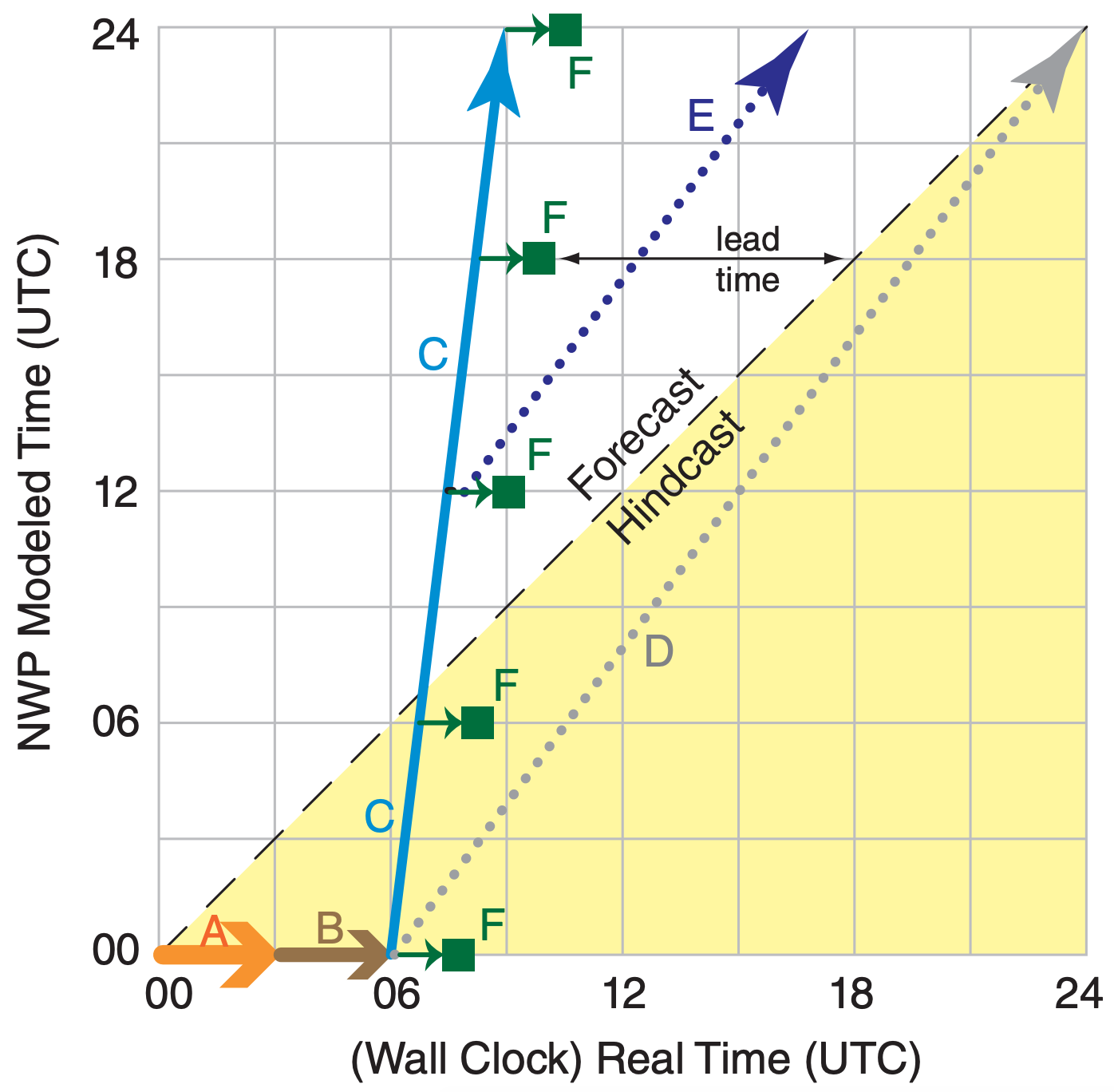
Fig. 20.12 shows a hypothetical forecast schedule, for a weather forecast initialized from 00 UTC synoptic observations. First, it takes a few hours (timeline A in Fig. 20.12) for all the data to be communicated from around the world to the weather forecast center (WFC). This step includes quality control, and rejection of suspected bad data.
Next, the data assimilation programs run for a few hours (B) to create a gridded analysis field. This is the optimum initial condition for the NWP model. At this point, we are ready to start making the forecast, but the initial conditions are already 6 h old compared to the present weather.
So the first part of forecast (C) is spent trying to catch up to “present”. This wasted initial forecast period is not lamented, because startup problems associated with the still-slightly-imbalanced initial conditions yield preliminary results that should be discarded anyway. Forecasts that occur AFTER the weather has already happened are known as hindcasts, as shown by the shaded area in Fig. 20.12.
The computer continues advancing the forecast (C) by taking small time steps. As the NWP forecast reaches key times, such as 6, 12, 18, and 24 (=00) UTC, the forecast fields are saved for post-processing and display (F). Lead time is how much the forecast is ahead of real time. For example, for coarse-mesh model (C), weather-map products (F) that are produced for a valid time of 18 UTC appear with a lead time of about 8 h before 18 UTC actually happens, in this hypothetical illustration.
Fig. 20.12 shows a coarse-mesh model (C) that takes 3 h of computation for each 24 h of forecast, as indicated by the slope of line (C). A finer-mesh model might take longer to run (with gentler slope). Model (D) takes 18 h to make a 24 h forecast, and if initialized from the 00 UTC initial conditions, might never catch up to the real weather during Day 1. Hence, it would be useless as a forecast — it would never escape from the hindcast domain.
But for one-way nesting, a fine-mesh forecast (E) could be initialized from the 12 UTC coarse-mesh forecast. This is analogous to a multi-stage rocket, where the coarse mesh (C) blasts the forecast from the past to the future, and then the finer-mesh (E) can remain in the future even though E has the same slope as D.
NWP meteorologists always have the need for speed. Faster computers allow most phases of the forecast process to run faster, allowing finer-resolution forecasts over larger domains with more accuracy and greater lead time. Speed-up can also be achieved computationally by making the dynamics and physics subroutines run faster, by utilizing more processor cores, and by utilizing special computer chips such as Graphics Processing Units (GPUs). However, tremendous speed-up of a few subroutines might cause only a small speed-up in the overall run time of the NWP model, as explained by Amdahl’s Law (see INFO Box).
The actual duration of phases (A) through (F) vary with the numerical forecast center, depending on their data-assimilation method, model numerics, domain size, grid resolution, and computer power. Details of the forecast phases are explained next.
Computer architect Gene Amdahl described the overall speedup factor SALL of a computer program as a function of the speedup Si of individual subroutines, where Pi is the portion of the total computation done by subroutine i:
\(\ S_{A L L}=\left[\sum\left(P_{i} / S_{i}\right)\right]^{-1}\)
and where ΣPi = 1.
Special programs called profilers can find how much time it takes to run each component of an NWP model, such as for the implementation of the Weather Research & Forecast (WRF) model shown below.
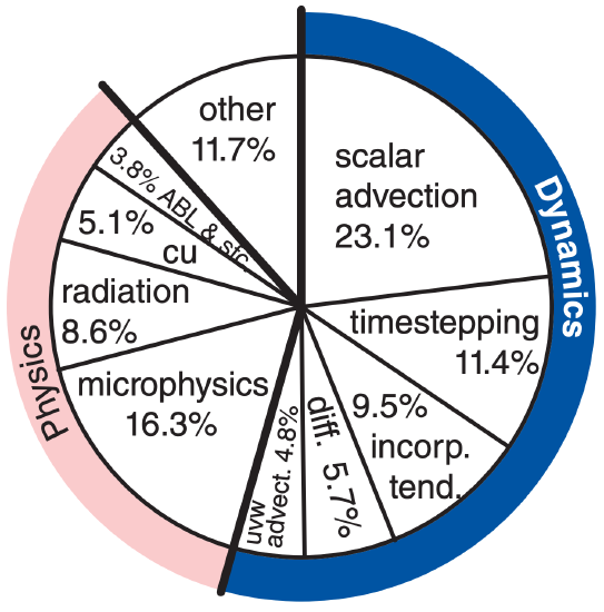
For example, if graphics-processing units (GPUs) speed up the microphysics 20 times and speed up scalar advection by 1.8 times (i.e., an 80% speedup), and the remaining 60.6% of WRF has no speedup, then overall:
SALL = [0.163/20 + 0.231/1.8 + 0.606/1]–1 = 1.35
Namely, even though the microphysics portion of the model is sped up 2000%, the overall speedup of WRF is 35% in this hypothetical example.
20.5.1. Balanced Mass and Flow Fields
Over the past few decades, it has been learned by experience that numerical models give bad forecasts if they are initialized from raw observed data. One reason is that the in-situ observation network has large gaps, such as over the oceans and in much of the Southern Hemisphere. Also, while there are many observations at the surface, there are fewer in-situ observations aloft. Remote sensors on satellites do not observe many of the needed dynamic variables (U, V, W, T, rT, ρ) directly, and have very poor vertical resolution. Observations can also contain errors, and local flow around mountains or trees can cause observations that are not representative of the larger-scale flow.
The net effect of such gaps, errors, and inconsistencies is that the numerical representation of this initial condition is imbalanced. By imbalanced, we mean that the observed winds disagree with the theoretical winds. An example of a theoretical wind is the geostrophic wind, which is based on temperature and pressure fields via atmospheric dynamics.


Balanced and imbalanced flows can be illustrated with a pond of water. Suppose initially the water-level is everywhere level, and the water currents and waves are zero (Fig. 20.13a). This flow system is balanced, because with a level pond surface we indeed expect no currents or waves. Next, add extra water to the center of the pond (Fig. 20.13b). This mass field (i.e., the distribution of water mass in the pond) is not balanced with the flow field (i.e., the motions or circulations within the pond, which for Fig. 20.13b are assumed to be zero). This imbalance causes waves and currents to form (Fig. 20.13c), which help to redistribute mass. These transient waves and currents decay, leaving the pond in a new balanced state (i.e., level water surface, no waves, no currents), but with slightly greater water depth.
Consider what happens to a numerical model of the pond if observation errors are incorporated into the initial conditions. Suppose that the water level in the center of the numerical pond is erroneously “observed” to be 1 m higher than the level everywhere else (Fig. 20.13b). Namely, the “true” initial conditions might be like Fig. 20.13a, but observation errors might cause the “modeled” initial conditions to be like Fig. 20.13b.
A well-designed numerical model of a pond would simulate the dynamical behavior of an actual pond. Hence, the modeled pond would respond as in Figs. 20.13c & d, even though the actual pond would remain motionless as in Fig. 20.13a.
The transient waves and currents are an artifact of the poor initial conditions in the model, and are not representative of the true flow in the real pond. Hence, the forecast results are not to be trusted during the first few minutes of the forecast period while the model is adjusting itself to a balanced state.
Numerical forecasts of the atmosphere have the same problem, but on a longer time scale than a pond. Namely, the first 0.5 to 3 hours of a weather forecast are relatively useless while the model adjusts to imbalances in the initial conditions (see the Data Assimilation section). During this startup period, simulated atmospheric waves are bouncing around in the model, both vertically and horizontally.
After the first 3 to 12 h of forecast, the dynamics are fairly well balanced, and give essentially the same forecast as if the fields were balanced from the start. However, spurious waves in the model might also cause unjustified rejection of good data during data assimilation (see next subsection).
Also, the erroneous waves can generate erroneous clouds that cause erroneous precipitation, etc. The net result could be an unrealistic loss of water from the model that could reduce the chance of future cloud formation and precipitation. Change of water content is just one of many irreversible processes that can permanently harm the forecast.
In summary, initialization problems cause a transient period of poor forecast quality, and can permanently degrade longer-term forecast skill or cause rejection of good data. Data-assimilation methods (described next) attempt to reduce startup imbalances, and are an important part of NWP.
20.5.2. Data Assimilation and Analysis
One hazard of data assimilation is that the resulting analysis does not represent truth, because the analysis includes a previous forecast as a first guess. If the previous forecast was wrong, then the subsequent analysis is poor.
Even worse are situations where there are little or no observation data. For data-sparse regions, the first-guess from the previous forecast dominates the “analysis”. This means that future forecasts start from old forecasts, not from observations. Forecast errors tend to accumulate and amplify, causing very poor forecast skill further downstream.
One such region is over the N.E. Pacific Ocean. From Fig. 9.23 in the Weather Reports & Map Analysis chapter, there are no rawinsonde observations (RAOBs) in that region to provide data at the dynamically important mid-tropospheric altitudes. Ships and buoys provide some surface data, and aircraft and satellites provide data near the tropopause, but there is a sparsity of data in the middle. This is known as the Pacific data void.
Poor forecast skill is indeed observed downstream of this data void, in British Columbia, Canada, and Washington and Oregon, USA. The weather-forecast difficulty there is exacerbated by the complex terrain of mountains and shoreline.
NWP forecast maps make up an important part of most weather briefings, but they should not be the only part. Bosart (2003), Snelling (1982), West (2011), and others recommend the following:
Your discussion should answer 6 questions:
- What has happened?
- Why has it happened?
- What is happening?
- Why is it happening?
- What will happen?
- Why will it happen?
Identify forecast issues throughout your briefing:
- Difficult/tricky forecast details.
- Significant/interesting weather.
Go from the large scale to the smaller scales.
Verify your previous forecast.
Encourage questions, discussion, and debate.
For the past and current weather portions of the briefing, show satellite images/animations, radar images/animations, soundings, and weather analyses.
Speak clearly, concisely, loudly, and with confidence. No forecast is perfect, but do the best you can. Your audience will appreciate your sincerity.
The technique of incorporating observations into the model’s initial conditions is called data assimilation (DA). Most assimilation techniques capitalize on the tendency of NWP models to create a balanced state during their forecasts.
One can utilize the balanced state from a previous forecast as a first guess of the initial conditions for a new forecast. When new weather observations are incorporated with the first guess, the result is called a weather analysis.
To illustrate the initialization process, suppose a forecast was started using initial conditions at 00 UTC, and that a 6-hour forecast was produced, valid at 06 UTC. This 06 UTC forecast could serve as the first guess for new initial conditions, into which the new 06 UTC weather observations could be incorporated. The resulting 06 UTC analysis could then be used as the initial conditions to start the next forecast run. The process could then be repeated for successive forecasts started every 6 h.
Although the analysis represents current or recent-past weather (not a forecast), the analyzed field is usually not exactly equal to the raw observations because the analysis has been smoothed and partially balanced. Observations are used as follows.
First, an automated initial screening of the raw data is performed. During this quality control phase, some observations are rejected because they are unphysical (e.g., negative humidities), or they disagree with most of the surrounding observations. In locations of the world where the observation network is especially dense, neighboring observations are averaged together to make a smaller number of statistically-robust observations.
When incorporating the remaining weather observations into the analysis, the raw data from various sources are not treated equally. Some sources have greater likelihood of errors, and are weighted less than those observations of higher quality. Also, observations made slightly too early or too late, or made at a different altitude, are weighted less. In some locations such as the tropics where Coriolis force and pressure gradients are weak, more weight can be given to the winds than to the pressures.
We focus on two data-assimilation methods here: optimum-interpolation DA and variational DA. Both are objective analysis methods in the sense that they are calculated by computer based on equations, in contrast to a “subjective analysis” by a human (such as was demonstrated in the Map Analysis chapter).
20.5.2.1. Objective optimum interpolation
| Table 20-2. Standard deviation σo of observation errors. | |
| Sensor Type | σo |
|---|---|
|
Wind errors in the lower troposphere: Surface stations and ship obs Drifting buoy Rawinsonde, wind profiler Aircraft and satellite |
(m s–1) 3 to 4 5 to 6 0.5 to 2.7 3 |
|
Pressure errors: Surface weather stations & Rawinsonde Ship and drifting buoy S. Hemisphere manual analysis |
(kPa) 0.1 0.2 0.4 |
|
Geopotential height errors: Surface weather stations Ship and drifting buoy S. Hemisphere manual analysis Rawinsonde |
(m) 7 14 32 13 to 26 |
|
Temperature errors: Automated Surface Obs. System (ASOS) Rawinsonde upper-air obs at z < 15 km at altitudes near 30 km |
(°C) 0.5 to 1.0 0.5 < 1.5 |
|
Humidity errors: ASOS surface weather stations: Td (°C) Rawinsonde in lower troposph: RH (%) near tropopause: RH (%) |
0.6 to 4.4 5 15 |
Let σo be the standard deviation of raw-observation errors from a sensor such as a rawinsonde (Table 20-2). Larger σ indicates larger errors.
Let σf be the standard deviation of errors associated with the first guess from a previous forecast. These are also known as background errors. Generally, error increases with increasing forecast range. For example, some global NWP models have the following errors for geopotential height Z of the 50-kPa isobaric surface:
\begin{align}\sigma_{Z f}=a \cdot t\tag{20.19}\end{align}
where a ≈ 11 m day–1 and t is forecast time range. Namely, a first guess from a 2-day forecast is less accurate (has greater error) than a first guess from a 1-day forecast.
An optimum interpolation analysis weights the first guess F and the observation O according to their errors to produce an analysis field A:
\begin{align}A=F \cdot \frac{\sigma_{0}^{2}}{\sigma_{f}^{2}+\sigma_{0}^{2}}+O \cdot \frac{\sigma_{f}^{2}}{\sigma_{f}^{2}+\sigma_{0}^{2}}\tag{20.20}\end{align}
where A, F, O , and σ all apply to the same one weather element, such as pressure, temperature, or wind. If the observation has larger errors than the first guess, then the analysis weights the observation less and the first-guess more.
Sample Application
A drifting buoy observes a wind of M = 10 m s–1, while the first guess for the same location gives an 8 m s–1 wind with 2 m s–1 likely error. Find the analysis wind speed.
Find the Answer
Given: MO = 10 m s–1, MF = 8 m s–1, σf = 2 m s–1
Find: MA = ? m s–1
Use Table 20-2 for Wind Errors: Drifting buoy: σo = 6 m s–1
Use eq. (20.20) for wind speed M:
\(\ M_{A}=M_{F} \cdot \frac{\sigma_{o}^{2}}{\sigma_{f}^{2}+\sigma_{o}^{2}}+M_{O} \cdot \frac{\sigma_{f}^{2}}{\sigma_{f}^{2}+\sigma_{o}^{2}}\)
\(\ M_{A}=(8 \mathrm{m} / \mathrm{s}) \cdot \frac{(6 \mathrm{m} / \mathrm{s})^{2}}{(2 \mathrm{m} / \mathrm{s})^{2}+(6 \mathrm{m} / \mathrm{s})^{2}}+(10 \mathrm{m} / \mathrm{s}) \cdot \frac{(2 \mathrm{m} / \mathrm{s})^{2}}{(2 \mathrm{m} / \mathrm{s})^{2}+(6 \mathrm{m} / \mathrm{s})^{2}}\)
= (8 m s–1)·(36/40) + (10 m s–1)·(4/40) = 8.2 m s–1
Check: Units OK. Physics OK.
Exposition: Because the drifting buoy has such a large error, it is given very little weight in producing the analysis. If it had been given equal weight as the first guess, then the average of the two would have been 9 m s–1. It might seem disconcerting to devalue a real observation compared to the artificial value of the first guess, but it is needed to avoid startup problems.
The equation above can be used to define a cost function J:
\begin{align}J(A)=\frac{1}{2}\left[\frac{(F-A)^{2}}{\sigma_{f}^{2}}+\frac{(O-A)^{2}}{\sigma_{o}^{2}}\right]\tag{20.21}\end{align}
where the optimum analysis from eq. (20.20) gives the minimum cost for eq. (20.21). An analysis (A) is bad (i.e., costly) if A differs greatly from F and O.
Optimum interpolation is “local” in the sense that it considers only the observations near a grid point when producing an analysis for that point. Also, optimum interpolation is not perfect, leaving some imbalances that cause atmospheric gravity waves to form in the subsequent forecast. A normal-mode initialization modifies the analysis further by removing the characteristics that might excite gravity waves.
20.5.2.2. Variational data assimilation
Another scheme, called variational analysis, attempts to match secondary characteristics calculated from the analysis field to observations so as to minimize the cost function. For example, the radiation emitted by air of the analyzed temperature is compared to radiance measured by satellite, allowing corrections to be made to the temperature analysis as appropriate.
Eq. (20.21) can be modified to utilize such secondary observations:
\begin{align}J(A)=\frac{1}{2}\left[\frac{(F-A)^{2}}{\sigma_{f}^{2}}+\frac{(Y-H(A))^{2}}{\sigma_{y 0}^{2}}\right]\tag{20.22}\end{align}
where H is an operator that converts from the analysis variable A to the secondary observed variable Y, and σyo is the standard deviation of observation errors for variable Y. The “best” analysis A is the one that minimizes the value of the cost function J. This minimum can be found by an iterative approach, or by trial and error.
For example, suppose a satellite radiometer looks toward Paris, and measures the upwelling radiance L for an infrared wavelength λ corresponding to the water-vapor channel of Fig. 8.8 in the Satellites & Radar chapter. This channel has the strongest returns at about 8 km altitude. For this example, Y is the measured radiance L. H(A) is the Planck blackbody radiance function (eq. 8.1), and A is the analysis temperature at 8 km over Paris. To find the best analysis, guess different values of A, calculate the associated cost function values, and iterate towards the value of A that yields the lowest value of cost function.
The variational approach allows you to consider all worldwide observations at the same time — a method called 3DVar. To do this, the first-guess (F), analysis (A), and observation (O) factors in eq. (20.22) must be replaced by vectors (arrays of numbers) containing all grid points in the whole 3-D model domain, and all observations made worldwide at the analysis time. Also, the first-guess and observation error variances must be replaced by covariance matrices. Although the resulting matrix-equation version of (20.22) contains millions of elements, large computers can iterate towards a “best” analysis.
An extension is 4DVar, where the additional dimension is time. This allows off-time observations to be incorporated into the variational analysis. 4DVar is even more computationally expensive than 3DVar. Although the role of any analysis method is to create the initial conditions for an NWP forecast, often it takes more computer time and power to create the optimum initial conditions than to run the subsequent numerical forecast.
Sample Application
The water vapor channel of a satellite observes a radiance of 1.53 W·m–2·µm–1·sr–1 over Paris. On average, this channel has an error standard deviation of 0.05 W·m–2·µm–1·sr–1. Output from a previous NWP run gives a temperature of –35°C at altitude 8 km over Paris, which we can use as a balanced first guess for the new analysis. This forecast has an error standard deviation of 1°C. The upper troposphere over Paris is very humid. For your analysis, find the “best” estimate of the temperature at 8 km over Paris.
Find the Answer
Given: Lo = 1.53 W·m–2·µm–1·sr–1 , TF = –35°C at 8 km
σLo = 0.05 W·m–2·µm–1·sr–1 , σTf = 1°C , watervapor channel: λ = 6.7 µm from the Satellites & Radar chapter with peak weighting function at z ≈ 8 km. High humidity implies blackbody emissions.
Find: TA = ? °C at 8 km altitude over Paris.
Use eq. (20.22), & use Planck’s Law eq. 8.1 for H(TA)
\(\ J\left(T_{A}\right)=\frac{1}{2}\left\{\frac{\left(T_{F}-T_{A}\right)^{2}}{\sigma^{2}_{T f}}+\frac{1}{\sigma_{L_{0}}^{2}}\left[L_{o}-\frac{c_{1 B} \cdot \lambda^{-5}}{\exp \left(\frac{c_{2}}{\lambda \cdot T_{A}}\right)-1}\right]^{2}\right\}\)
with c1B = 1.191043x10⁸ W·m–2·µm4·sr–1 and c2 = 14387.75 µm K from near eq. (8.1) in The Satellites & Radar chapter. [Hint: don’t forget to convert TA in Kelvin to use in Planck’s Law.]
Calculate J(TA) for various values of TA. I will start with a std. atmosphere guess of TA = –37°C at 8 km.
J = 0.5 · { [(–35°C)–(–37°C)]2/(1°C)2 + (1/(0.05u)2 ·[1.53u – (8822u/(exp(9.09926) – 1)) ]2 }
J = 0.5 ·{ 4 + 118.4 } = 61.2 (dimensionless)
where u are units of W·m–2·µm–1·sr–1.
Repeating the calculation in a spreadsheet for other values of TA in the range of –37 to –25°C gives:
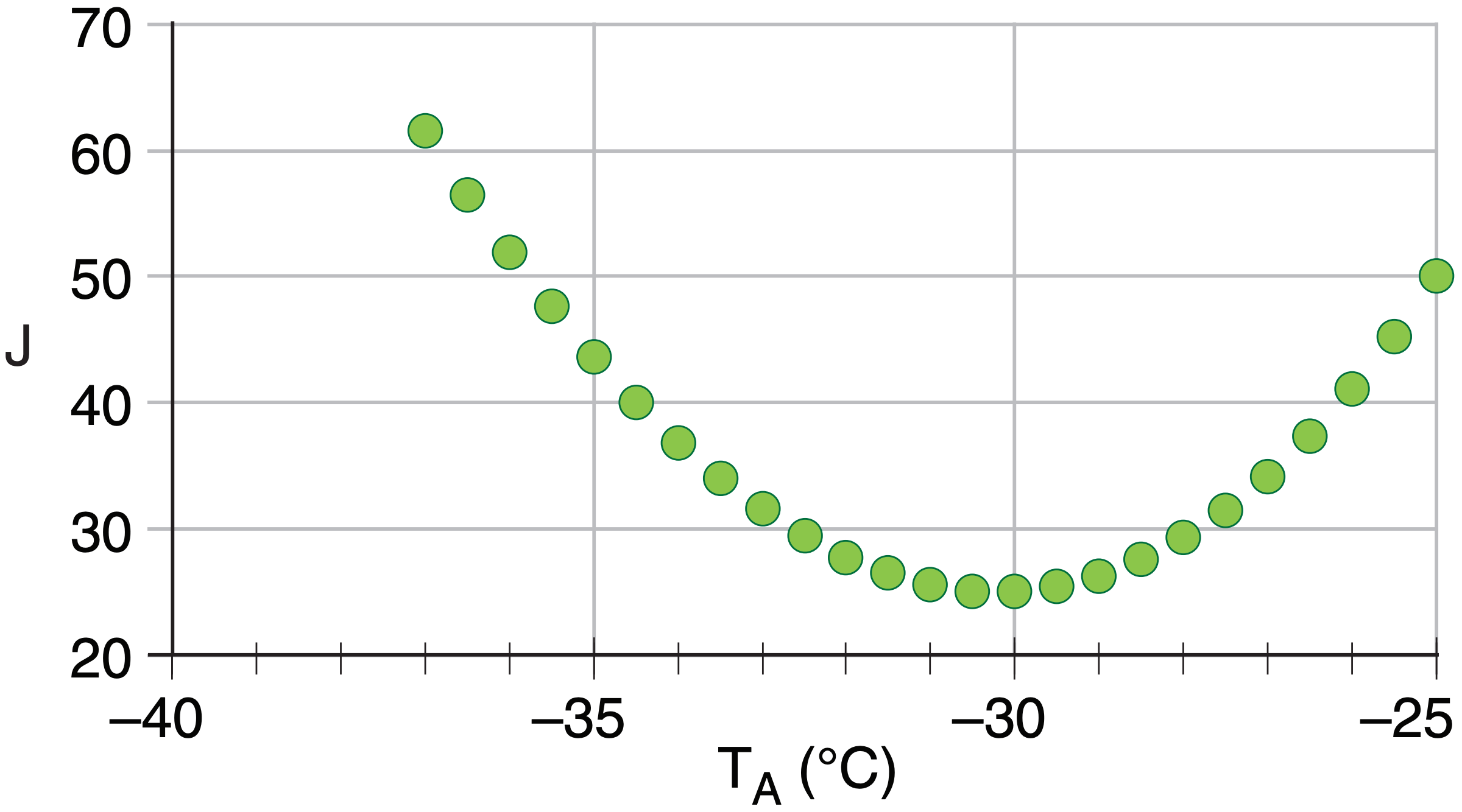
The best analysis is at minimum cost J, near TA= –30°C
Check: Units OK. TA value reasonable.
Exposition: The satellite radiance corresponds to a brightness temperature of –25°C. An error propagation calculation (see Appendix A) for eq. (8.1) shows that a radiance error of σLo = 0.05 W·m–2·µm–1·sr–1 corresponds to a brightness-temperature error of 1°C. Thus, both the first guess and the observed radiance have the same effective error, giving TA equally weighted between the satellite value –25°C and the first-guess value –35°C. Try different error values in the spreadsheet to see how TA varies between –35 & –25°C
20.5.3. Forecast
| Table 20-3. Hierarchy of operational numerical weather prediction (NWP) models. | ||
| Forecast Type | Fcst. Duration & (Fcst. Cycle) | Domain & (∆X) |
|---|---|---|
| nowcasts | 0 to 3 h (re-run every few minutes) | local: town, county (100s of m) |
| short-range | 3 h to 3 days (re-run every few hours) | regional: state, national, continental (1 to 5 km) |
| medium-range | 3 to 7 days (re-run daily) | continental to global (5 to 25 km) |
| long-range | 7 days to 1 month (re-run daily or weekly) | global (25 to 100 km) |
| seasonal | 1 to 12 months (re-run monthly) | global (100 to 500 km) |
| GCM* | 1 to 1000 years [non-operational (not run routinely); focus instead on case studies & hypothetical scenarios.] | global (100 to 500 km |
* GCM = Global Climate Model -or- General Circulation Model.
The next phase of the forecast process is the running of the NWP models. Recall that weather consists of the superposition of many different scales of motion (Table 10-6), from small turbulent eddies to large Rossby waves. Different NWP models focus on different time and spatial scales (Table 20-3).
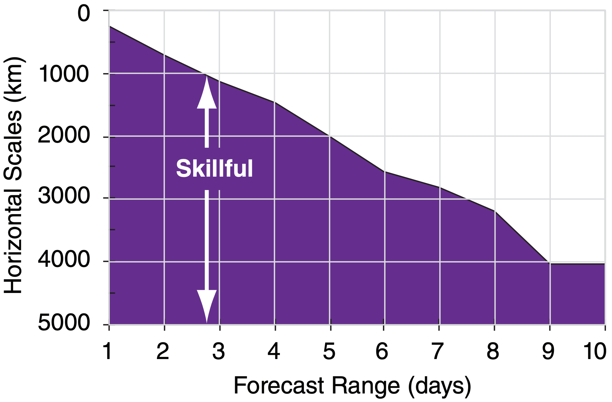
Unfortunately, the forecast quality of the smaller scales deteriorates much more rapidly than that for the larger scales. For example, cloud forecasts might be good out to 2 to 12 hours, frontal forecasts might be good out to 12 to 36 hours, while the Rossby-wave forecasts might be useful out to several days. Fig. 20.14 indicates the ranges of horizontal scales over which the forecast is reasonably skillful.
Don’t be deceived when you look at a weather forecast, because all scales are superimposed on the weather map regardless of the forecast duration. Thus, when studying a 5 day forecast, you should try to ignore the small features on the weather map such as thunderstorms or frontal positions. Even though they exist on the map, they are probably wrong. Only the positions of the major ridges and troughs in the jet stream might possess any forecast skill at this forecast duration. Maps in the next section illustrate such deterioration of small scales.
20.5.4. Case Study: 22-25 Feb 1994
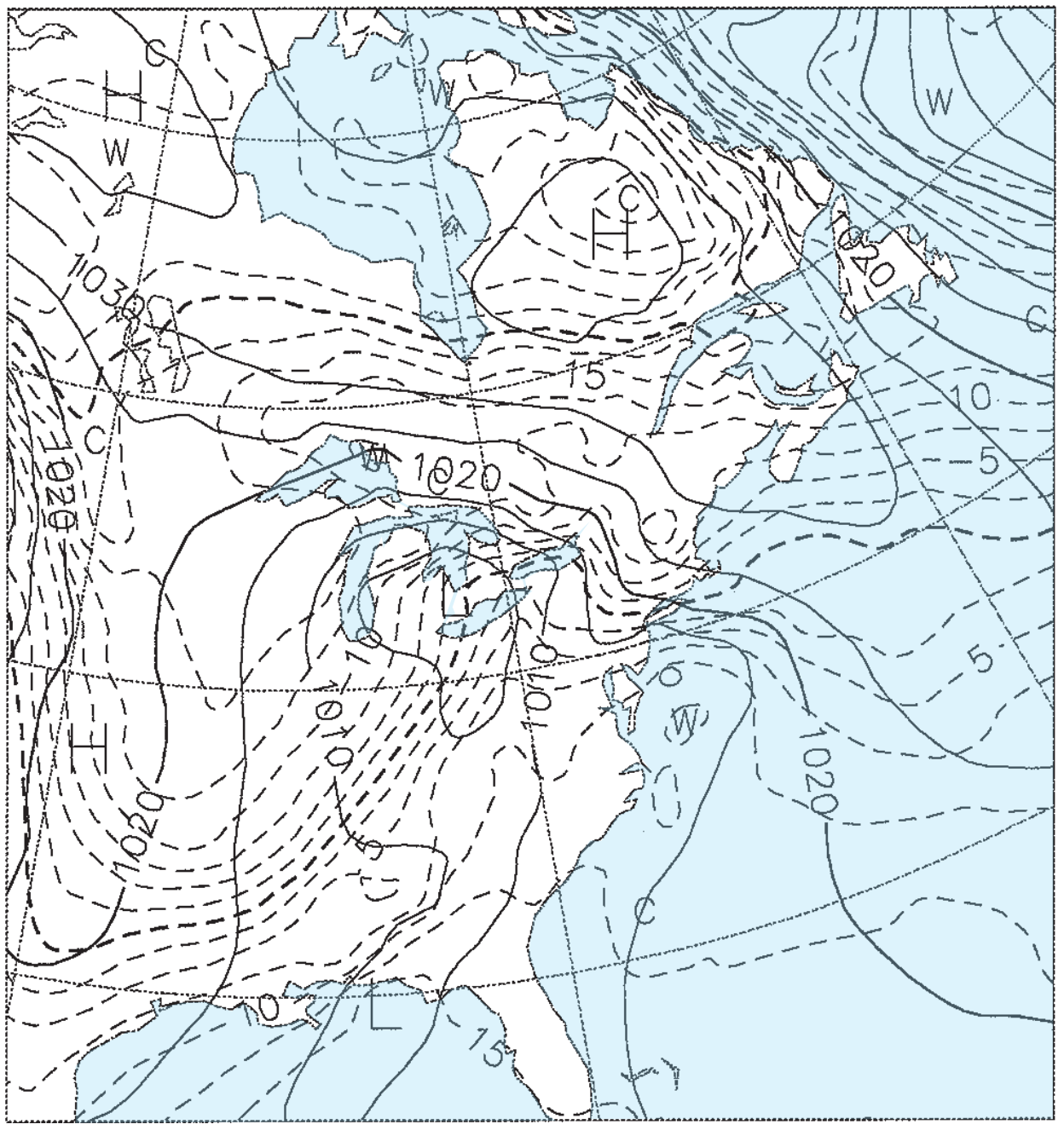
Figs. 20.15b-e give the weather forecasts valid for the same time, but initialized 1.5, 3.5, 5.5, and 7.5 days earlier. For example, Fig. 20.15b was initialized with weather observations from 12 UTC on 22 Feb 94, and the resulting 1.5 day forecast valid at 00 UTC on 24 Feb 94 is shown in the figure. Fig. 20.15c was initialized from 12 UTC on 20 Feb 94, and the resulting 3.5 day forecast is shown in the figure. Thus, each succeeding figure is the result of a longer-range forecast, which started with earlier observations, but ended at the same time.
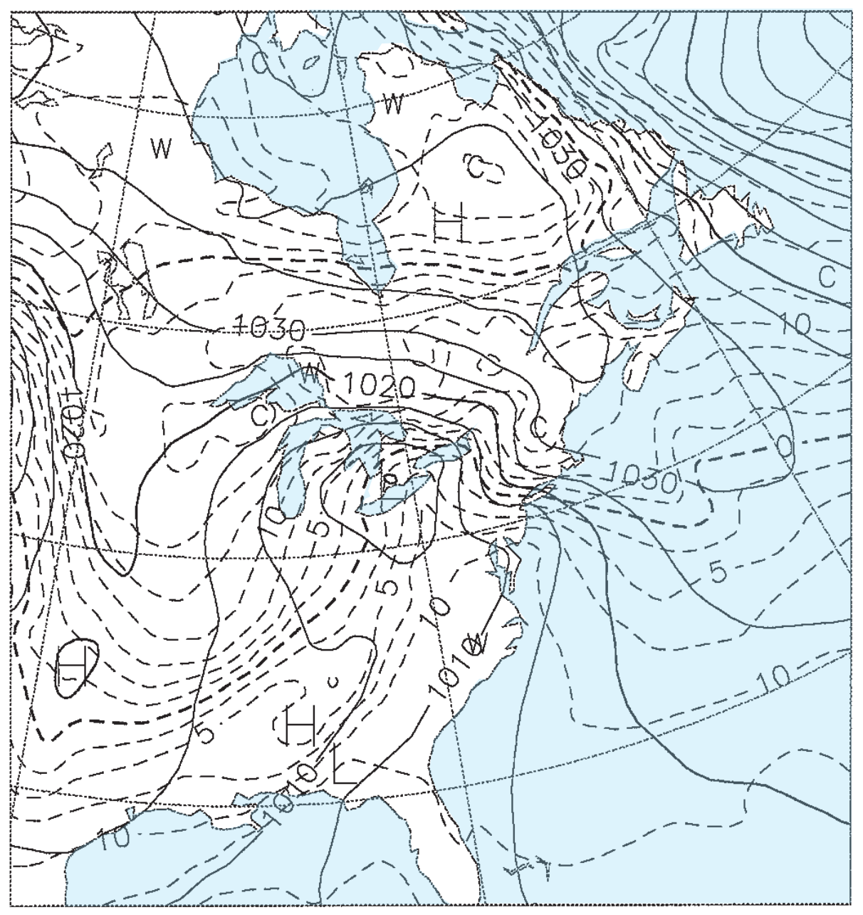
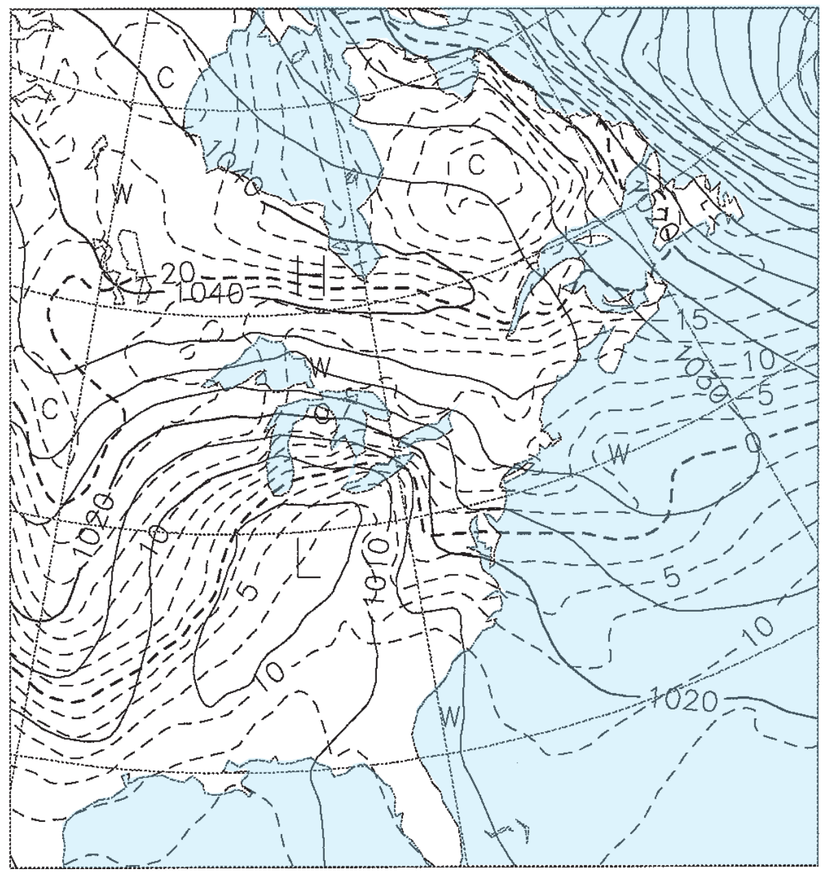
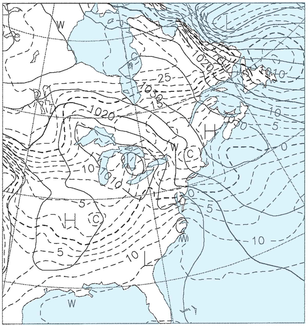
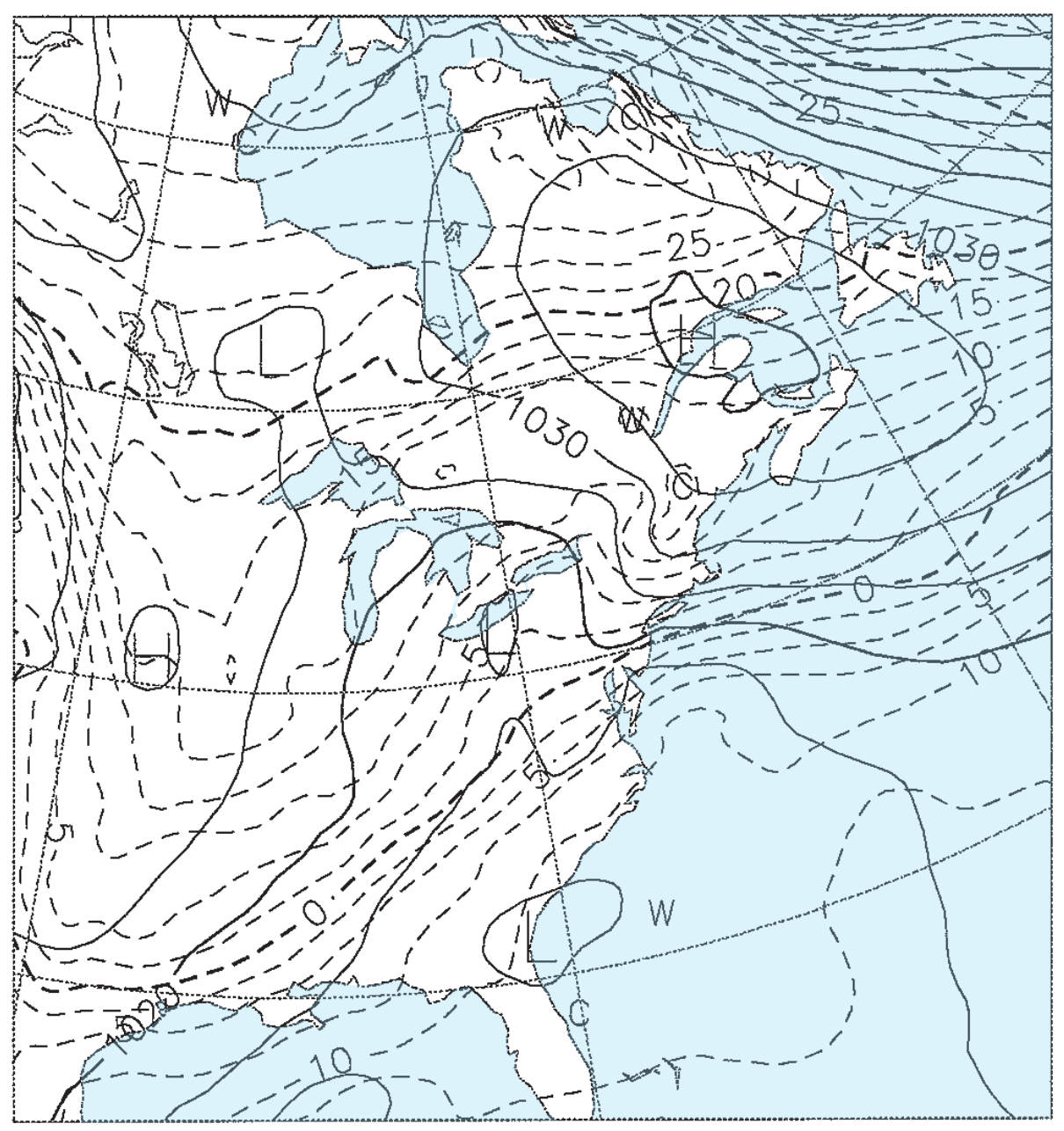
Solid isobars are MSL pressure in mb (1000 mb = 100 kPa), plotted every 5 mb. Dashed isotherms are 85-kPa temperatures, plotted every 2.5°C, with the 0°C line darker. The map domain covers eastern North America, and is centered on Lake Ontario.
These figures demonstrate the inconsistency of forecasts started at different times with different initial conditions. Such inconsistency is inherent in all forecasts, and illustrates the limits of predictability. The analysis (Fig. 20.15a) shows a low centered near Detroit, Michigan, with a cold front extending southwest toward Arkansas. The 1.5-day forecast (Fig. 20.15b) is reasonably close, but the 3.5-day forecast (Fig. 20.15c) shows the low too far south and the cold front too far west. The 5.5 and 7.5-day forecasts (Fig. 20.15d & e) show improper locations for the fronts and lows, but larger-scale features are good.
20.5.5. Post-processing
Suppose that y represents a weather element observed at a weather station. Let x be the corresponding forecast by a NWP model. Over many days, you might accumulate many (N) data points (xi , yi ) of forecasts and corresponding observations, where i is the data-point index.
If you anticipate that the relationship between x and y is linear, then that relationship can be described by:
\(\ y=a_{0}+a_{1} \cdot x\)
where ao is an unknown bias (called the intercept), and a1 is an unknown trend (called the slope).
The best-fit (in the least-squared-error sense) coefficients are:
\(\ a_{o}=\frac{(\bar{x}) \cdot \overline{x y}-\overline{x^{2}} \cdot(\bar{y})}{(\bar{x})^{2}-\overline{x^{2}}} \quad \quad \quad \quad \quad \quad a_{1}=\frac{(\bar{x}) \cdot \bar{y}-\overline{x y}}{(\bar{x})^{2}-\overline{x^{2}}}\)
The overbar indicates an average over all data points of the quantity appearing under the overbar; e.g.:
\bar{x}=\frac{1}{N} \sum_{i=1}^{N} x_{i} \quad \quad \quad \quad\overline{x y}=\frac{1}{N} \sum_{i=1}^{N}\left(x_{i} \cdot y_{i}\right) \quad \quad \quad \quad \overline{x^{2}}=\frac{1}{N} \sum_{i=1}^{N}\left(x_{i}^{2}\right)
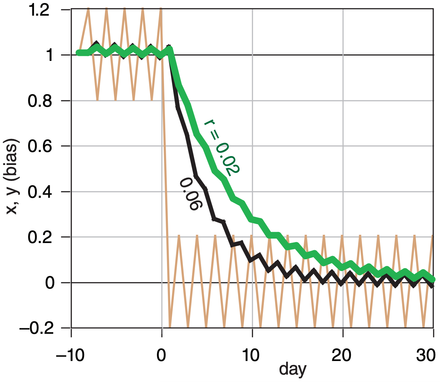
Rudolf Kalman suggested a method that we can modify to estimate the bias x in tomorrow’s forecast. It uses the observed bias y in today’s forecast, and also uses yesterday’s estimate for today’s bias xold:
\(\ x=x_{\text {old }}+\beta \cdot\left(y-x_{\text {old }}\right)\)
The Kalman gain β depends on ratio r = σ2PL/σ2NWP , where σ2 PL is the “predictability-limit” error variance associated with the chaotic nature of a “perfect” weather-forecast model, and σ2NWP is the error variance of the operational NWP model. If those error variances are steady, then β = 0.5·[(r2+4r)1/2 – r]. The e-folding response time (days) is τ = –1/[ln(1–β)].
Midlatitude weather is more variable and less predictable in winter. As a result, useful values are:
- Winter: r ≈ 0.06 , β = 0.217 , \(\ \tau\) = 4 days.
- Summer: r ≈ 0.02 , β = 0.132 , \(\ \tau\) = 7 days.
This Fig. shows a noisy input y (thin tan line) & KF responses x (thicker lines) for different values of the ratio r. The KF adapts to changes, and is recursive.
After the dynamical computer model has completed its forecast, additional post-processing computations can be made with the saved output. Post-processing can include:
- forecast refinement to correct biases,
- calculation of secondary weather variables,
- drawing of weather maps and other graphics,
- compression into databases & climatologies, &
- verification (see the Forecast Quality section).
20.5.5.1. Forecast Refinement
Forecasts often contain biases (systematic errors; see Appendix A), due to the NWP model formulation, the initial conditions used, and characteristics of different locales. For example, towns might be located in valleys or near coastlines. These are landscape features that can modify the local weather, but which might not be captured by a coarse-mesh numerical model. A number of automated statistical techniques (e.g., linear regression, Kalman filtering) can be applied as post-processing to reduce the biases and to tune the model output toward the climatologically-expected or observed local weather.
Two classical statistical methods are the Perfect Prog Method (PPM) and Model Output Statistics (MOS). Both methods use a best-fit statistical regression (see INFO boxes) to relate input fields (predictors) to different output fields (predictands). An example of a predictand is surface temperature at a weather station, while predictors for it might include values interpolated from the nearest NWP grid points. PPM uses observations as predictors to determine regression coefficients, while MOS uses model forecast fields. Once the regression coefficients are found, both methods then use the model forecast fields as the predictors to find the surfacetemperature forecast for that weather station.
Best-fit regressions are found using multi-year sets of predictors and predictands. The parameters of the resulting best-fit regression equations are held constant during their subsequent usage.
The PPM method has the advantage that it does not depend on the particular forecast model, and can be used immediately after changing the forecast model. The PPM produces best predictand values (e.g., of secondary variables) only when the model produces perfect predictor forecasts, which is rare.
The MOS advantage is that any systematic model errors can be compensated by the statistical regression. A disadvantage of MOS is that a multi-year set of model output must first be collected and statistically fit, before the resulting regression can be used for future forecasts. Both MOS and PPM have a disadvantage that the statistical parameters are fixed.
Alternative methods include the Kalman Filter (KF; see INFO box) and Updateable MOS, which continually refine their statistical parameters each day. They share the advantage of MOS in that they use model output for the predictors. They learn from their mistakes (i.e., are adaptive), and can automatically and quickly re-tune themselves after any changes in the numerical model or in the synoptic conditions. They are recursive (tomorrow’s bias correction depends on today’s bias correction, not on many years of past data), which significantly reduces the data-storage requirements. A disadvantage is that the KF cannot capture rare, extreme events.
Sample Application (§)
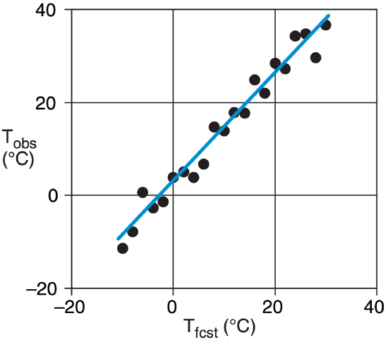
Given the following set of past data (Tfcst vs. Tobs): (a) Find the best-fit straight line. Namely, train MOS using linear regression (see Linear Regr. INFO box). (b) If the NWP forecast for tomorrow is Tfcst = 15°C, then post-process it to estimate the bias-corrected T ?
Find the Answer
Given: The first 3 columns of data below.
Find: ao = ? °C, a1 = ? , Tfcst = ? °C
(a) Train MOS using past data to find the coefficients.
| i | x=Tfcst | y=Tobs | x·y | x2 |
|
1 2 3 4 5 6 7 8 9 10 11 12 13 14 15 16 17 18 19 20 21 |
-10 -8 -6 -4 -2 0 2 4 6 8 10 12 14 16 18 20 22 24 26 28 30 |
-11.4 -7.9 0.7 -2.7 -1.4 3.8 5.0 3.8 6.7 14.7 13.9 17.9 17.7 24.8 22.0 28.4 27.2 34.3 34.7 29.7 36.7 |
114.0 62.8 -4.0 10.9 2.8 0.0 10.1 15.2 40.0 117.5 139.1 214.3 247.8 397.0 396.4 568.0 599.5 822.0 902.7 831.1 1100.3 |
100 64 36 16 4 0 4 16 36 64 100 144 196 256 324 400 484 576 676 784 900 |
| avg= | 10.0 | 14.2 | 313.7 | 246.7 |
ao = (10 · 313.7 – 246.7 · 14.2) / (102 – 246.7) = 2.52 °C
a1 = ( 10 · 14.2 – 313.7 ) / (102 – 246.7) = 1.17 (dim’less)
The original data points and the best-fit line are:
(b) Use MOS to correct the forecast: T = ao + a1 · Tfcst . T = (2.52°C) + 1.17·(15°C) = 20.1 °C.
Check: Units OK. Line fits data nicely.
Exposition: The predictor (x) and predictand (y) need not have the same units. For example, MOS could be trained to use model forecasts of relative humidity (%) to estimate observed values of visibility (km).
If you draw a vertical line from each data point to the regressed line, then the length of each line is a measure of the error between the data and the regression. Square each error value and sum them to give the total error. Linear regression is a “best fit” in the sense of finding the “least squared error”.
20.5.5.2. Calculation of Secondary Variables
Fundamental output from the NWP forecast include winds, temperature, pressure or height, mixing ratio, and precipitation. Additional weather variables can be created for human forecasters, for the general public, and for specific industries such as agriculture, transportation, and utilities. Some of these secondary variables (such as relative humidity) can be calculated directly from the primary fields using their defining equations. Other secondary variables (such as visibility) can be estimated statistically via regression.
Secondary thermodynamic variables include: potential temperature, virtual potential temperature, liquid-water or equivalent potential temperature, wet-bulb temperature, near-surface (z = 2 m) temperature, surface skin temperature, surface heat fluxes, surface albedo, wind-chill temperature, static stability, short- and long-wave radiation, and various storm-potential indices such as CAPE.
Secondary moisture variables include: relative humidity, cloudiness (altitudes and coverage), precipitation type and amount, visibility, near-surface dew-point (z = 2 m), soil wetness, and snowfall.
Secondary dynamic variables include streamlines, trajectories, absolute vorticity, potential vorticity, isentropic potential vorticity, dynamic tropopause height, vorticity advection, Richardson number, dynamic stability, near-surface winds (z = 10 m), surface stress, surface roughness, mean sea-level pressure, and turbulence.
While many of the above variables are computed at central numerical-computing facilities, additional computations can be made by separate organizations. For example, local weather-forecast offices can tailor the numerical guidance from national NWP centers to produce local forecasts of maximum and minimum temperature, precipitation, cloudiness, and storm and flood warnings.
Other organizations such as consulting firms, broadcast companies, utility companies, and airlines can acquire the fundamental and secondary fields via data networks such as the internet. From these fields they compute products such as computerized flight plans for aircraft, crop indices and threats such as frost, hours of sunshine, and heating- or cooling-degree days for energy consumption.
Universities also acquire the primary and secondary output fields, to use for teaching and research. Some of the applications result in weather maps that are put back on the internet.
20.5.5.3. Weather Maps and Other Graphics
The fundamental and secondary variables that are output from the NWP and from forecast refinement are arrays of numbers. To make these data easier to use and interpret by humans, the numbers can be converted into weather-map graphics and animations, meteograms (plots of a weather variable vs. time), sounding profiles, cross-sections, text forecasts, and other output forms. Computation of these outputs can take hours, depending on the graphical complexity and the number of products, and thus cannot be neglected in the forecast schedule.
Some visualization programs for NWP output include: GrADS, Vis5D, MatLab, NCAR RIP, GEMPAK, Vapor, IDV, AWIPS, NinJo & WINGRIDDS.
20.5.5.4. Compression into Databases and Climatologies
It is costly to save the terabytes of output produced by operational NWP models every day for every grid point, every level, and every time step. Instead, only key weather fields at RAOB mandatory levels in the atmosphere are saved. These WMO standard isobaric surfaces are: surface, 100, 92.5, 85, 70, 50, 40, 30, 25, 20, 15, 10, 7, 5, 3, 2, & 1 kPa. Output files can be converted from model-specific formats to standard formats (NetCDF, Vis5D, SQL, GRIB). Forecasts at key locations such as weather stations can be accumulated into growing climatologies.
Sample Application
Given the following simplified MOS regression:
\(\ T_{\min }=-295+0.4 \cdot T_{15}+0.25 \cdot \Delta T H+0.6 \cdot T_{d}\)
for daily minimum temperature (K) in winter at Madison, Wisconsin, where T15 = observed surface temperature (K) at 15 UTC, ∆TH = model forecast of 100- 85 kPa thickness (m), and Td = model fcst. dew point (K). Predict Tmin given NWP model forecasts of: T15 = 273 K, ∆TH = 1,200 m, and Td = 260 K.
Find the Answer
Given: T15 = 273 K, ∆TH = 1,200 m, and Td = 260 K.
Find: Tmin = ? K
Tmin = –295 + 0.4·(273) + 0.25·(1,200)+ 0.6·(260) = 270.2 ≈ –3°C.
Check: Units OK. Physics OK.
Exposition: Chilly, but typical for winter in Madison. Note that MOS regressions can be made for any variables in any units. Thus, (1) units might not be consistent from term to term in the regression, but (2) you MUST use the same units for each variable as was used when the MOS regression was created.
In their 2015 paper, P. Bauer, A. Thorpe and G. Brunet reviewed “The quiet revolution of numerical weather prediction.” Nature (doi:10.1038/nature14956).
“Revolution” in the sense that NWP has mostly superseded humans in its ability to rapidly collect and quality-control observations, make analyses, make forecasts, produce weather maps, write the text of weather forecasts, track NWP skill, save climatologies, adjust the forecasts to locales, tailor outputs of secondary variables, and disseminate it all via the internet.
“Quiet” in the sense that the forecast skill improvements happened gradually over many decades.
As a result of the shrinking advantage of human forecasters over NWP, the role of the meteorologist is changing. Some countries don’t allow their government meteorologists to modify the automated forecast, or limit the changes that are allowed.
Instead, modern meteorologists interpret the NWP output to relate it to human needs (food, water, energy), safety, and social conditions. Meteorologists use NWP forecasts to help make decisions in weather-dependent industries and insurance, to analyze effects of storms and climate change that relate to engineering design and building-code policy, to anticipate where clean-energy facilities could be built, and to improve transportation safety and commerce.
University curricula are changing to reflect these new roles. We still teach the physics and dynamics of how the weather works. But we increasingly emphasize the social aspects interpreting, applying, and communicating the NWP forecasts.


