20.2: Grid Points
- Page ID
- 9660

\( \newcommand{\vecs}[1]{\overset { \scriptstyle \rightharpoonup} {\mathbf{#1}} } \)
\( \newcommand{\vecd}[1]{\overset{-\!-\!\rightharpoonup}{\vphantom{a}\smash {#1}}} \)
\( \newcommand{\id}{\mathrm{id}}\) \( \newcommand{\Span}{\mathrm{span}}\)
( \newcommand{\kernel}{\mathrm{null}\,}\) \( \newcommand{\range}{\mathrm{range}\,}\)
\( \newcommand{\RealPart}{\mathrm{Re}}\) \( \newcommand{\ImaginaryPart}{\mathrm{Im}}\)
\( \newcommand{\Argument}{\mathrm{Arg}}\) \( \newcommand{\norm}[1]{\| #1 \|}\)
\( \newcommand{\inner}[2]{\langle #1, #2 \rangle}\)
\( \newcommand{\Span}{\mathrm{span}}\)
\( \newcommand{\id}{\mathrm{id}}\)
\( \newcommand{\Span}{\mathrm{span}}\)
\( \newcommand{\kernel}{\mathrm{null}\,}\)
\( \newcommand{\range}{\mathrm{range}\,}\)
\( \newcommand{\RealPart}{\mathrm{Re}}\)
\( \newcommand{\ImaginaryPart}{\mathrm{Im}}\)
\( \newcommand{\Argument}{\mathrm{Arg}}\)
\( \newcommand{\norm}[1]{\| #1 \|}\)
\( \newcommand{\inner}[2]{\langle #1, #2 \rangle}\)
\( \newcommand{\Span}{\mathrm{span}}\) \( \newcommand{\AA}{\unicode[.8,0]{x212B}}\)
\( \newcommand{\vectorA}[1]{\vec{#1}} % arrow\)
\( \newcommand{\vectorAt}[1]{\vec{\text{#1}}} % arrow\)
\( \newcommand{\vectorB}[1]{\overset { \scriptstyle \rightharpoonup} {\mathbf{#1}} } \)
\( \newcommand{\vectorC}[1]{\textbf{#1}} \)
\( \newcommand{\vectorD}[1]{\overrightarrow{#1}} \)
\( \newcommand{\vectorDt}[1]{\overrightarrow{\text{#1}}} \)
\( \newcommand{\vectE}[1]{\overset{-\!-\!\rightharpoonup}{\vphantom{a}\smash{\mathbf {#1}}}} \)
\( \newcommand{\vecs}[1]{\overset { \scriptstyle \rightharpoonup} {\mathbf{#1}} } \)
\( \newcommand{\vecd}[1]{\overset{-\!-\!\rightharpoonup}{\vphantom{a}\smash {#1}}} \)
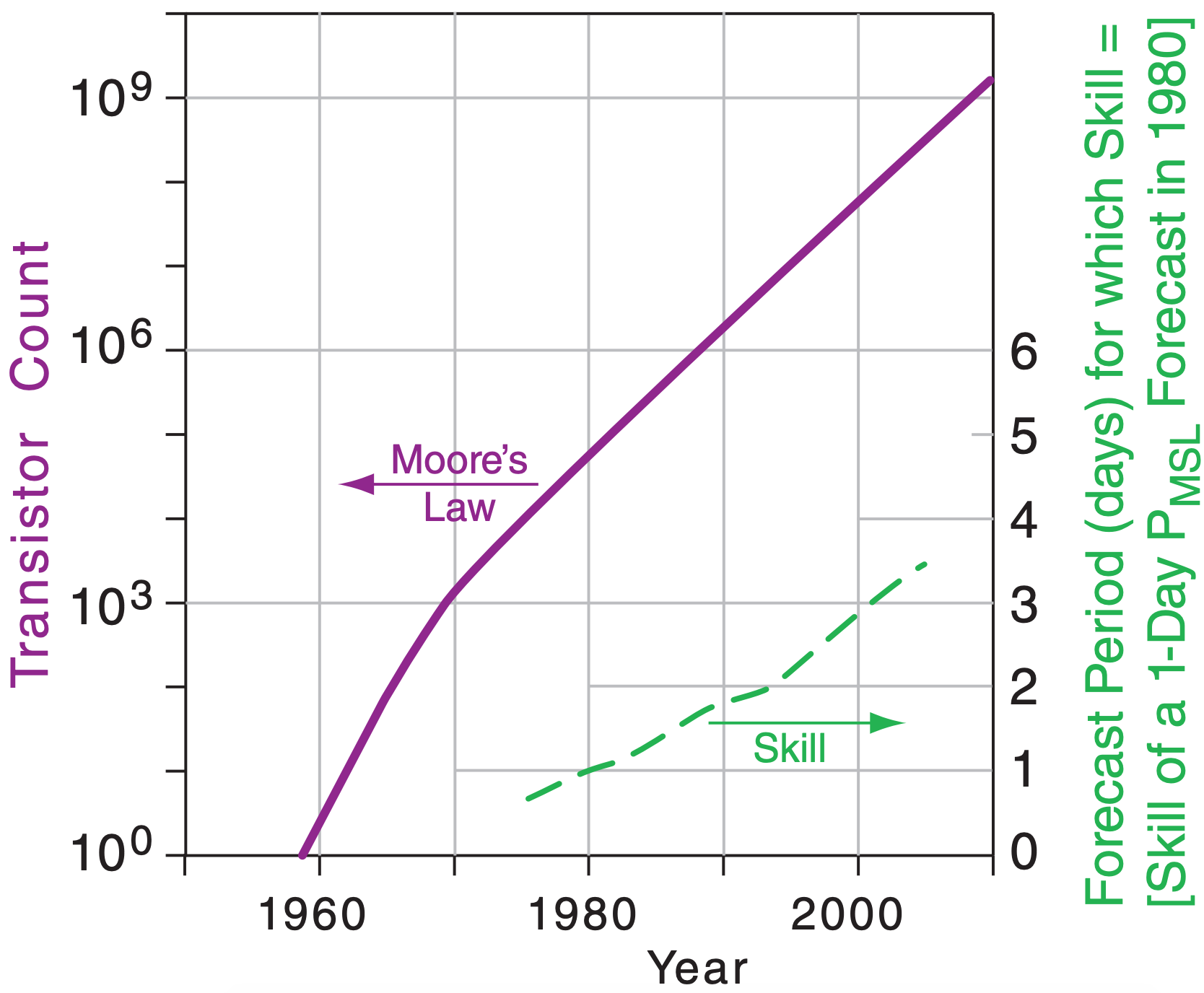
\(\newcommand{\avec}{\mathbf a}\) \(\newcommand{\bvec}{\mathbf b}\) \(\newcommand{\cvec}{\mathbf c}\) \(\newcommand{\dvec}{\mathbf d}\) \(\newcommand{\dtil}{\widetilde{\mathbf d}}\) \(\newcommand{\evec}{\mathbf e}\) \(\newcommand{\fvec}{\mathbf f}\) \(\newcommand{\nvec}{\mathbf n}\) \(\newcommand{\pvec}{\mathbf p}\) \(\newcommand{\qvec}{\mathbf q}\) \(\newcommand{\svec}{\mathbf s}\) \(\newcommand{\tvec}{\mathbf t}\) \(\newcommand{\uvec}{\mathbf u}\) \(\newcommand{\vvec}{\mathbf v}\) \(\newcommand{\wvec}{\mathbf w}\) \(\newcommand{\xvec}{\mathbf x}\) \(\newcommand{\yvec}{\mathbf y}\) \(\newcommand{\zvec}{\mathbf z}\) \(\newcommand{\rvec}{\mathbf r}\) \(\newcommand{\mvec}{\mathbf m}\) \(\newcommand{\zerovec}{\mathbf 0}\) \(\newcommand{\onevec}{\mathbf 1}\) \(\newcommand{\real}{\mathbb R}\) \(\newcommand{\twovec}[2]{\left[\begin{array}{r}#1 \\ #2 \end{array}\right]}\) \(\newcommand{\ctwovec}[2]{\left[\begin{array}{c}#1 \\ #2 \end{array}\right]}\) \(\newcommand{\threevec}[3]{\left[\begin{array}{r}#1 \\ #2 \\ #3 \end{array}\right]}\) \(\newcommand{\cthreevec}[3]{\left[\begin{array}{c}#1 \\ #2 \\ #3 \end{array}\right]}\) \(\newcommand{\fourvec}[4]{\left[\begin{array}{r}#1 \\ #2 \\ #3 \\ #4 \end{array}\right]}\) \(\newcommand{\cfourvec}[4]{\left[\begin{array}{c}#1 \\ #2 \\ #3 \\ #4 \end{array}\right]}\) \(\newcommand{\fivevec}[5]{\left[\begin{array}{r}#1 \\ #2 \\ #3 \\ #4 \\ #5 \\ \end{array}\right]}\) \(\newcommand{\cfivevec}[5]{\left[\begin{array}{c}#1 \\ #2 \\ #3 \\ #4 \\ #5 \\ \end{array}\right]}\) \(\newcommand{\mattwo}[4]{\left[\begin{array}{rr}#1 \amp #2 \\ #3 \amp #4 \\ \end{array}\right]}\) \(\newcommand{\laspan}[1]{\text{Span}\{#1\}}\) \(\newcommand{\bcal}{\cal B}\) \(\newcommand{\ccal}{\cal C}\) \(\newcommand{\scal}{\cal S}\) \(\newcommand{\wcal}{\cal W}\) \(\newcommand{\ecal}{\cal E}\) \(\newcommand{\coords}[2]{\left\{#1\right\}_{#2}}\) \(\newcommand{\gray}[1]{\color{gray}{#1}}\) \(\newcommand{\lgray}[1]{\color{lightgray}{#1}}\) \(\newcommand{\rank}{\operatorname{rank}}\) \(\newcommand{\row}{\text{Row}}\) \(\newcommand{\col}{\text{Col}}\) \(\renewcommand{\row}{\text{Row}}\) \(\newcommand{\nul}{\text{Nul}}\) \(\newcommand{\var}{\text{Var}}\) \(\newcommand{\corr}{\text{corr}}\) \(\newcommand{\len}[1]{\left|#1\right|}\) \(\newcommand{\bbar}{\overline{\bvec}}\) \(\newcommand{\bhat}{\widehat{\bvec}}\) \(\newcommand{\bperp}{\bvec^\perp}\) \(\newcommand{\xhat}{\widehat{\xvec}}\) \(\newcommand{\vhat}{\widehat{\vvec}}\) \(\newcommand{\uhat}{\widehat{\uvec}}\) \(\newcommand{\what}{\widehat{\wvec}}\) \(\newcommand{\Sighat}{\widehat{\Sigma}}\) \(\newcommand{\lt}{<}\) \(\newcommand{\gt}{>}\) \(\newcommand{\amp}{&}\) \(\definecolor{fillinmathshade}{gray}{0.9}\)Gordon E. Moore co-founded the integrated-circuit (computer-chip) manufacturer Intel. In 1965 he reported that the maximum number of transistors that were able to be inexpensively manufactured on integrated circuits had doubled every year. He predicted that this trend would continue for another decade.
Since 1970, the rate slowed to about a doubling every two years. This trend, known as Moore’s Law, has continued for over 4 decades.
Increasing computer power has enabled improved NWP models that use finer grids covering larger areas with more-complicated physics and numerics. Thus NWP forecast skill has improved concomitant with computer power.
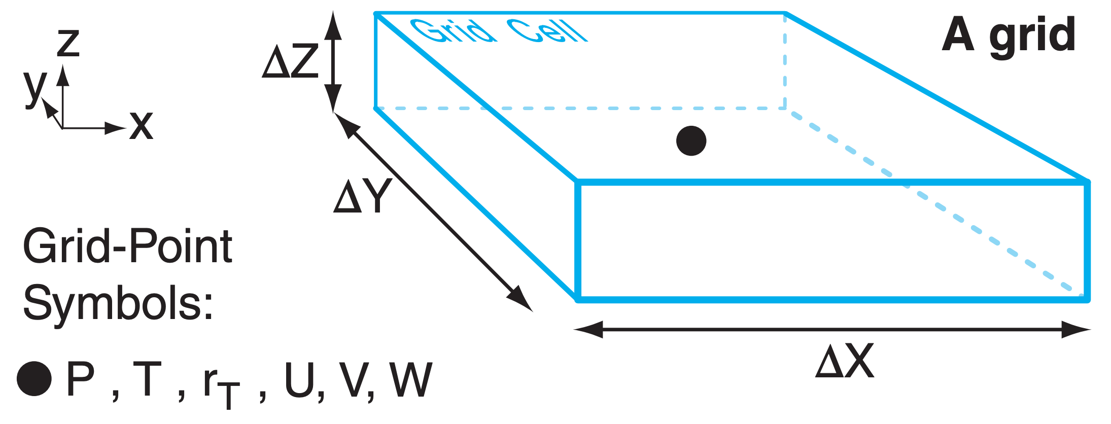
Define the size of a grid cell in the three Cartesian directions as ∆X, ∆Y, and ∆Z (Fig. 20.6A). Typical values are ∆X = ∆Y = one to hundreds of kilometers, while ∆Z = one to hundreds of meters. Small-size grid cells give fine-resolution (or high-resolution) forecasts, and large-size cells give coarse-resolution (or low-resolution) forecasts.
Because we forecast only the average condition of weather variables at each grid cell, we can represent these average values as being physically located at a grid point (Fig. 20.6A) in each cell. The distance between grid points is the same as the grid-cell size: ∆X, ∆Y, ∆Z. Grid points spaced more closely have finer resolution (see a later INFO Box on Resolution).
Finer resolution requires more grid cells to span your forecast domain. Each cell requires a certain number of numerical calculations to make the forecast. Thus, more cells require more total calculations. Hence, finer resolution forecasts take longer to compute, but often give more accurate forecasts.
Thus, your choice of domain and grid size is a compromise between forecast timeliness and accuracy, based on the computer power available. As computer power has improved over the past 6 decades, so have weather-forecast resolution and skill (see INFO Box on Moore’s Law and Forecast Skill). Skill (see section 20.7) is the forecast improvement relative to some reference such as climatology.
20.2.1. Nested and Variable Grids
 https://eoimages.gsfc.nasa.gov/images/ imagerecords/54000/54388/BlueMarble.jpg
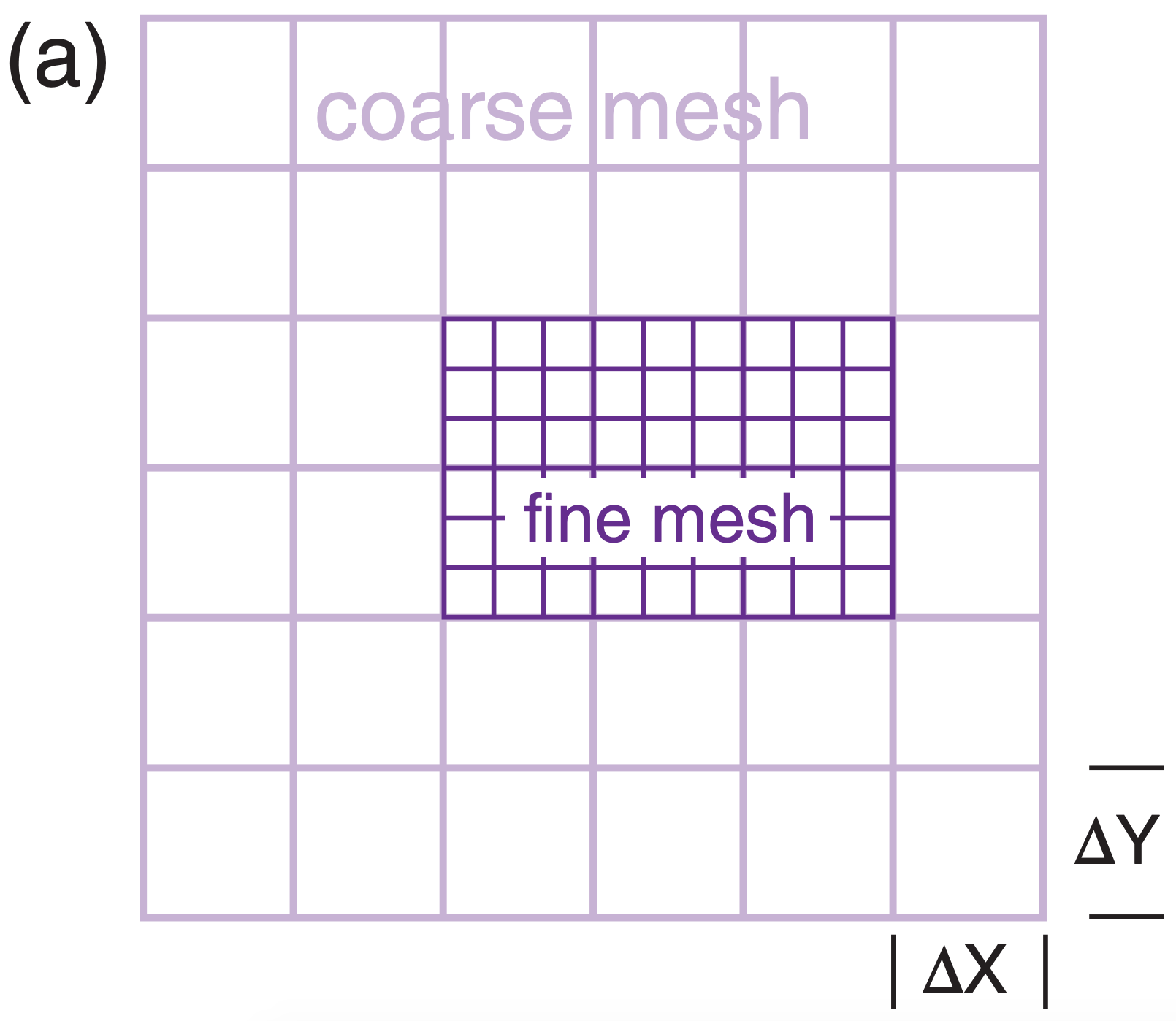
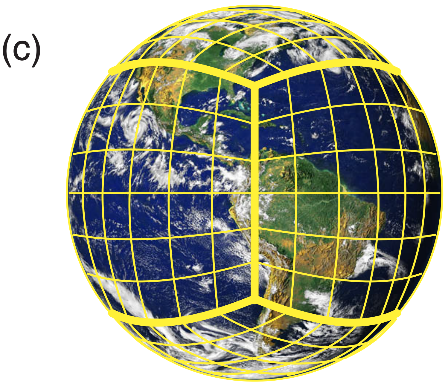
Modeling strategies have been devised to compensate for the domain-size vs. resolution trade off. In the horizontal, you can use a fast-running coarse grid over a large domain to span synoptic weather systems. Inside it, embed a smaller-domain finer-mesh nested grid (Fig. 20.4a) to capture mesoscale details where they are needed most. Typically, the fine mesh has a horizontal grid size (∆X) of 1/3 of the coarse-mesh grid size, although ratios of 1/5 have sometimes been used. (Odd numbers are used in the denominator to ensure that each coarse grid point coincides with a fine grid point.) Nesting can continue with successively finer nests. The author’s research team has run nested grids with grid sizes ∆X = 108, 36, 12, 4, 1.33, and 0.44 km.
Nested grids can employ one-way nesting, where the coarse grid is solved first, and its output is applied as time-varying boundary conditions to the finer grid. For two-way nesting, both grids are solved together, and features from each grid are fed into the other at each time step. Two-way nesting often gives better forecasts, but is more complicated to implement.
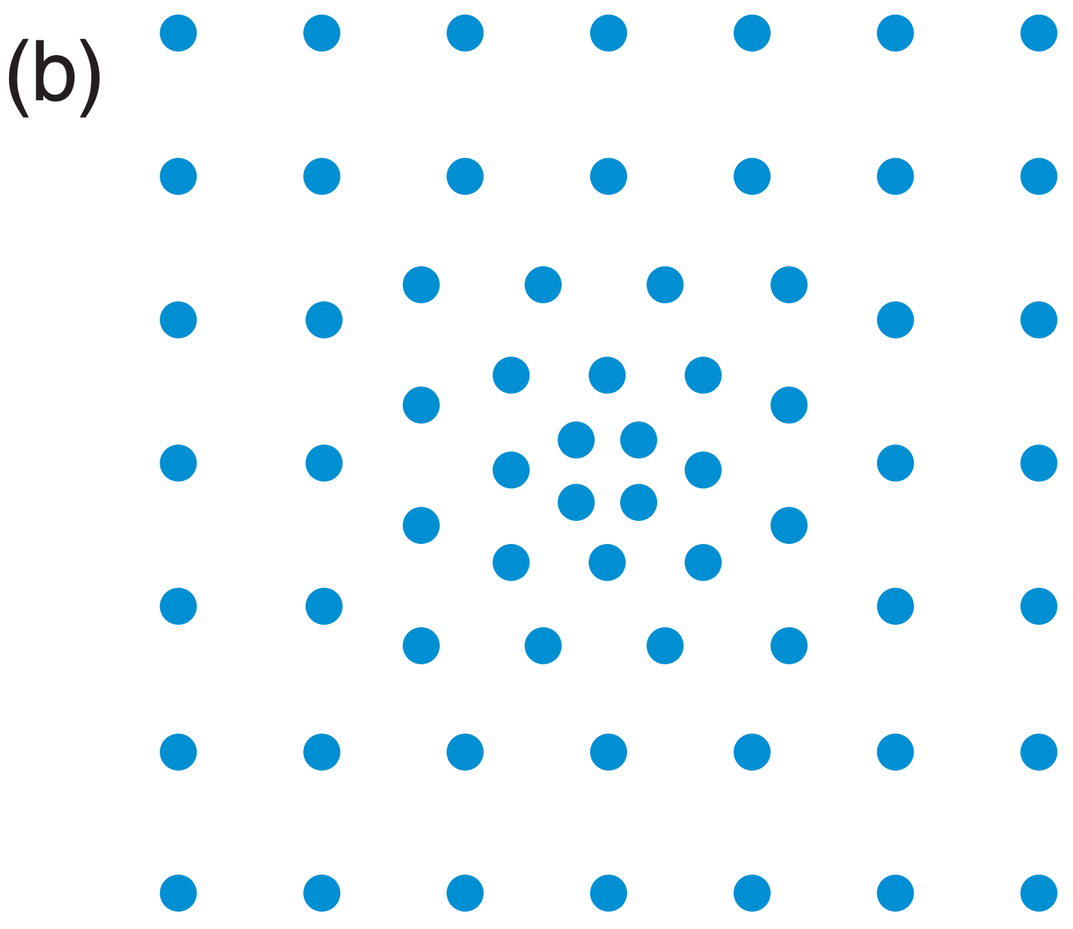
An alternative to discrete nested grids in the horizontal is a variable-mesh grid (Fig. 20.4b), which uses smoothly varying grid spacings. Again, the finer mesh is positioned over the region of interest.
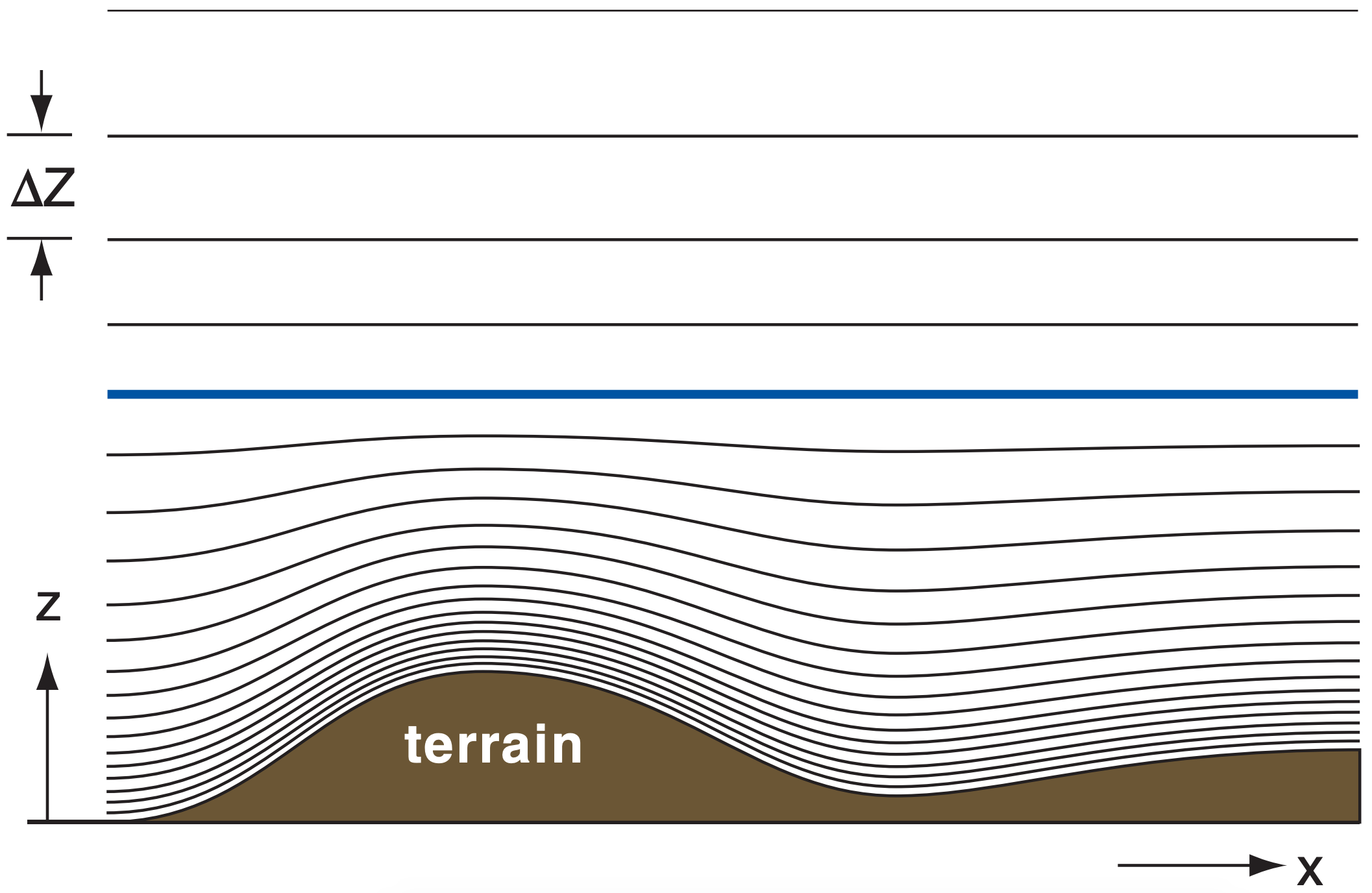
In the vertical, fine resolution (i.e., small ∆Z) is needed near the Earth’s surface and in the boundary layer, because of important small-scale motions and strong vertical gradients. To reduce the computation time, coarse resolution (i.e., larger ∆Z) is acceptable higher above the surface — in the stratosphere and upper troposphere. Variable mesh vertical grids (i.e., smoothly changing ∆Z values) are often used for this reason (Fig. 20.5). For models using pressure or sigma as a vertical coordinate, ∆P or ∆σ varies smoothly with height. As an alternative, some NWP models use discrete vertical nests.
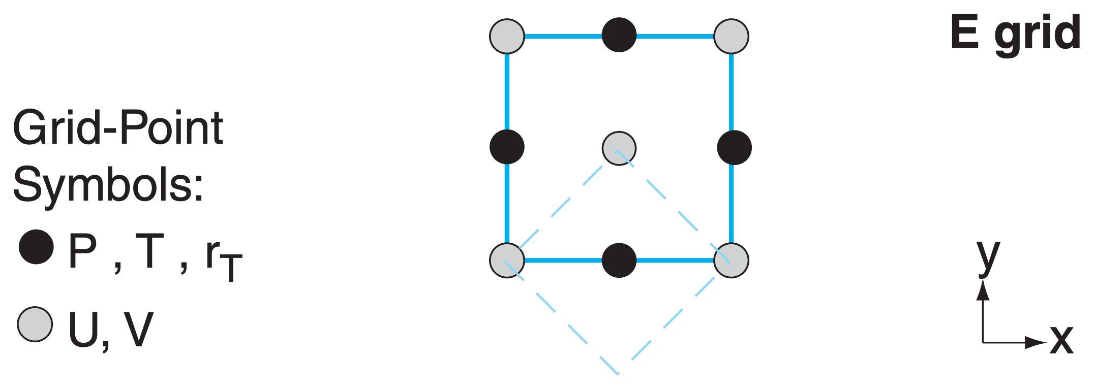
20.2.2. Staggered Grids
You could represent all the cell-averaged variables at the same grid point, as in Fig. 20.6A (called an A-Grid). But this has some undesirable characteristics: wavy motions do not disperse properly, some wave energy gets stuck in the grid, and some weather variables oscillate about their true value.
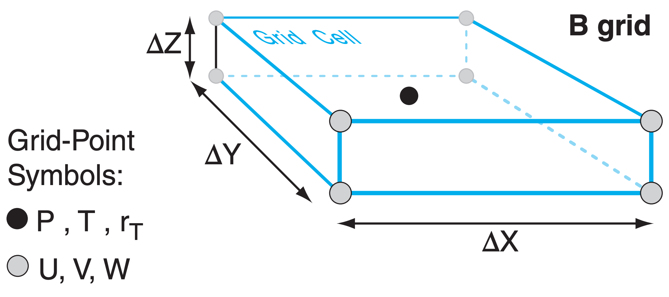
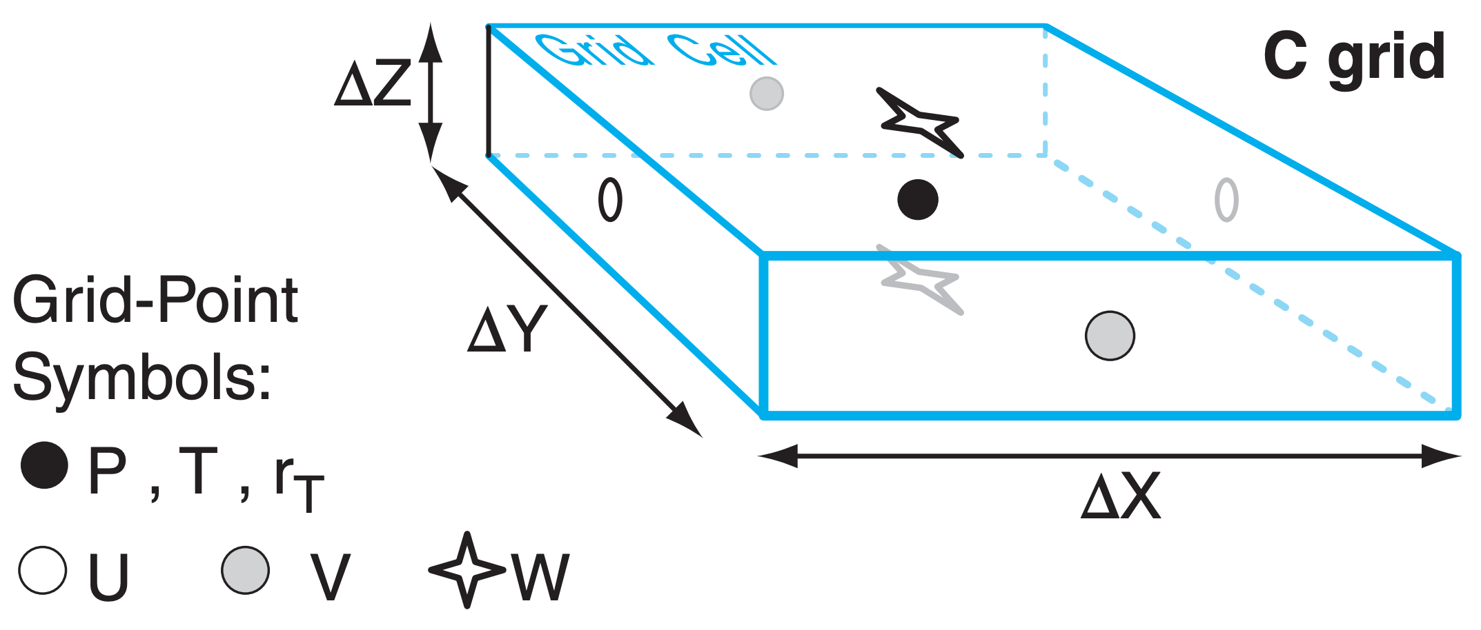
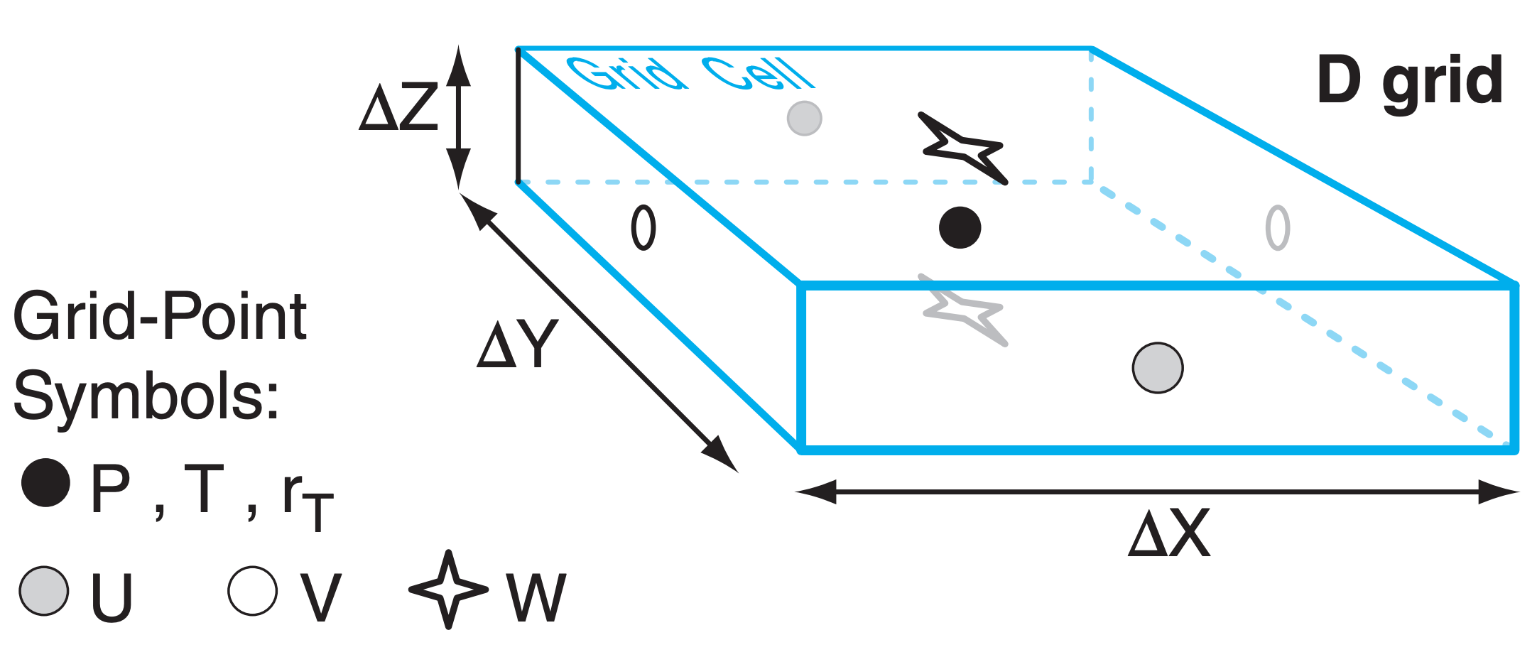
Instead, grid points are often arranged in a staggered grid arrangement within the cell, with different variables being represented by points at different locations in the grid (Fig. 20.6 Grids B - E). Staggered Grid D has many of the same problems as unstaggered Grid A. Grids B and C have fewer problems.