

19: Pollutant Dispersion
- Page ID
- 9658

\( \newcommand{\vecs}[1]{\overset { \scriptstyle \rightharpoonup} {\mathbf{#1}} } \)
\( \newcommand{\vecd}[1]{\overset{-\!-\!\rightharpoonup}{\vphantom{a}\smash {#1}}} \)
\( \newcommand{\dsum}{\displaystyle\sum\limits} \)
\( \newcommand{\dint}{\displaystyle\int\limits} \)
\( \newcommand{\dlim}{\displaystyle\lim\limits} \)
\( \newcommand{\id}{\mathrm{id}}\) \( \newcommand{\Span}{\mathrm{span}}\)
( \newcommand{\kernel}{\mathrm{null}\,}\) \( \newcommand{\range}{\mathrm{range}\,}\)
\( \newcommand{\RealPart}{\mathrm{Re}}\) \( \newcommand{\ImaginaryPart}{\mathrm{Im}}\)
\( \newcommand{\Argument}{\mathrm{Arg}}\) \( \newcommand{\norm}[1]{\| #1 \|}\)
\( \newcommand{\inner}[2]{\langle #1, #2 \rangle}\)
\( \newcommand{\Span}{\mathrm{span}}\)
\( \newcommand{\id}{\mathrm{id}}\)
\( \newcommand{\Span}{\mathrm{span}}\)
\( \newcommand{\kernel}{\mathrm{null}\,}\)
\( \newcommand{\range}{\mathrm{range}\,}\)
\( \newcommand{\RealPart}{\mathrm{Re}}\)
\( \newcommand{\ImaginaryPart}{\mathrm{Im}}\)
\( \newcommand{\Argument}{\mathrm{Arg}}\)
\( \newcommand{\norm}[1]{\| #1 \|}\)
\( \newcommand{\inner}[2]{\langle #1, #2 \rangle}\)
\( \newcommand{\Span}{\mathrm{span}}\) \( \newcommand{\AA}{\unicode[.8,0]{x212B}}\)
\( \newcommand{\vectorA}[1]{\vec{#1}} % arrow\)
\( \newcommand{\vectorAt}[1]{\vec{\text{#1}}} % arrow\)
\( \newcommand{\vectorB}[1]{\overset { \scriptstyle \rightharpoonup} {\mathbf{#1}} } \)
\( \newcommand{\vectorC}[1]{\textbf{#1}} \)
\( \newcommand{\vectorD}[1]{\overrightarrow{#1}} \)
\( \newcommand{\vectorDt}[1]{\overrightarrow{\text{#1}}} \)
\( \newcommand{\vectE}[1]{\overset{-\!-\!\rightharpoonup}{\vphantom{a}\smash{\mathbf {#1}}}} \)
\( \newcommand{\vecs}[1]{\overset { \scriptstyle \rightharpoonup} {\mathbf{#1}} } \)
\(\newcommand{\longvect}{\overrightarrow}\)
\( \newcommand{\vecd}[1]{\overset{-\!-\!\rightharpoonup}{\vphantom{a}\smash {#1}}} \)
\(\newcommand{\ket}[1]{\left| #1 \right>}\)
\(\newcommand{\bra}[1]{\left< #1 \right|}\)
\(\newcommand{\braket}[2]{\left< #1 \vphantom{#2} \right| \left. #2 \vphantom{#1} \right>}\)
\(\newcommand{\braopket}[3]{\left< #1 \vphantom{#2}\vphantom{#3} \right| #2 \vphantom{#1}\vphantom{#3} \left| #3 \vphantom{#1}\vphantom{#2} \right>}\)
\(\newcommand{\qmvec}[1]{\mathbf{\vec{#1}}}\)
\(\newcommand{\op}[1]{\hat{\mathbf{#1}}}\)
\(\newcommand{\expect}[1]{\langle #1 \rangle}\)
\(\newcommand{\dfn}[1]{\emph{\textbf{#1}}}\)
Every living thing pollutes. Life is a chemical reaction, where input chemicals such as food and oxygen are converted into growth or motion. The reaction bi-products are waste or pollution.
The only way to totally eliminate pollution is to eliminate life — not a particularly appealing option. However, a system of world-wide population control could stem the increase of pollution, allowing residents of our planet to enjoy a high quality of life.
Is pollution bad? From an anthropocentric point of view, we might say “yes”. To do so, however, would deny our dependence on pollution. In the Earth’s original atmosphere, there was very little oxygen. Oxygen is believed to have formed as pollution from plant life. Without this pollutant, animals such as humans would likely not exist now.
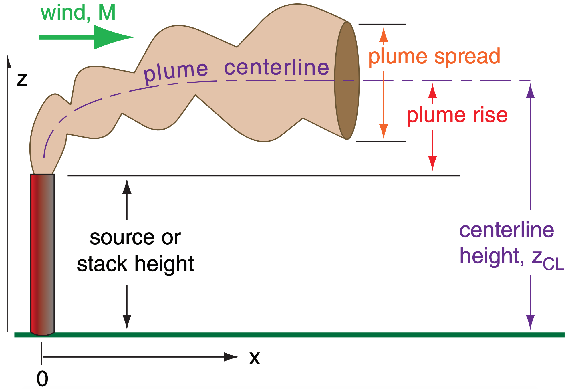
However, it is reasonable to worry about other chemicals that threaten our quality of life. We call such chemicals pollutants, regardless of whether they form naturally or anthropogenically (man-made). Many of the natural sources are weak emissions from large area sources, such as forests or swamps. Anthropogenic sources are often concentrated at points, such as at the top of smoke stacks (Fig. 19.1). Such high concentrations are particularly hazardous, and been heavily studied.
- 19.1: Dispersion Factors
- This page explores smoke plumes, differentiating between air pollution and atmospheric science definitions. It covers plume rise, dispersion factors (like wind speed and turbulence), and tracking pollutant concentrations using trajectory techniques. Measurement units for pollutants, such as parts per million and micrograms per cubic meter, are outlined.
- 19.2: Air Quality Standards
- This page discusses the establishment of air quality standards for managing air pollution in various countries, including NAAQS in the USA, CAAQS in Canada, and EU regulations. It details specific pollutant standards and notes that violations may arise from environmental factors or control issues. Additionally, it emphasizes the role of effective air pollution modeling in facility design to ensure compliance, suggesting potential adjustments when needed.
- 19.3: Turbulence Statistics
- This page explains the influence of mean wind speed and turbulence on pollutant dispersion from point sources. It highlights the importance of analyzing wind characteristics, distinguishing between mean and turbulent components, and introduces isotropy and anisotropy in turbulence.
- 19.4: Dispersion Statistics
- This page covers differences between instantaneous smoke plume snapshots and averaged representations, highlighting how snapshots reveal variability while averages yield a Gaussian concentration profile with a defined centerline height and standard deviation for plume spread.
- 19.5: Taylor's Statistical Theory
- This page covers plume dispersion in relation to turbulence and distance. It explains the diffusion equation for passive tracers, noting that dispersion increases over time based on turbulence intensity. The Gaussian solution and Taylor's statistical theory reveal how plume spread can be predicted.
- 19.6: Dispersion in Neutral and Stable Boundary Layers
- This page covers the calculation and modeling of pollutant concentrations from dispersion and plume rise. It explains how plume rise occurs due to momentum and buoyancy and varies in different atmospheric conditions, along with the use of Gaussian distribution models for concentration estimation. It also details dispersion models that consider turbulent velocity, plume spread, and receptor concentrations, while highlighting limitations in certain terrains.
- 19.7: Dispersion in Unstable Boundary Layers (Convective Mixed Layers)
- This page explores pollutant dispersion in a statically unstable boundary layer with light winds over warm surfaces. It details how thermals generate asymmetric turbulence affecting smoke dispersion from sources like stacks. The methodology includes normalizing variables with convective scales to measure plume height and concentration.
- 19.8: Review
- This page covers the dispersion of pollutants from smokestacks, highlighting the significance of stack height for pollution dilution and compliance with air-quality standards. It explains that air-quality assessments are based on average pollutant concentrations, modeled using statistical dispersion theories. The influence of turbulence on dispersion under varying atmospheric conditions is detailed, along with classification schemes for turbulence characteristics.
- 19.9. Homework Exercises
- This page provides an overview of exercises and discussions related to air pollution research, modeling, and dispersion. It encourages online research into regulatory agencies and pollution standards, while including practical calculations on pollutants and atmospheric conditions. Key concepts include plume modeling, dispersion equations, and the impact of environmental factors on air quality.