19.5: Taylor's Statistical Theory
- Page ID
- 9656
Statistical theory explains how plume dispersion statistics depend on turbulence statistics and downwind distance.
The Gaussian concentration distribution is a solution to the diffusion equation, as is shown here.
For a conservative passive tracer, the budget equation says that concentration c in a volume will increase with time t if greater tracer flux Fc enters the volume than leaves. In one dimension (z), this is:
\(\ \begin{align}\frac{d c}{d t}=-\frac{\partial F_{c}}{\partial z}\tag{a}\end{align}\)
If turbulence consists of only small eddies, then the turbulent flux of tracer flows down the mean tracer gradient:
\(\ \begin{align}F_{c}=-K \frac{\partial c}{\partial z}\tag{b}\end{align}\)
where K, the eddy diffusivity, is analogous to a molecular diffusivity (see K-Theory in the Atmospheric Boundary Layer chapter), and Fc is in kinematic units (concentration times velocity).
Plug eq. (b) into (a), and assume constant K to obtain the 1-D diffusion equation:
\(\ \begin{align}\frac{d c}{d t}=K \frac{\partial^{2} C}{\partial z^{2}}\tag{c}\end{align}\)
This parabolic differential equation can be solved with initial conditions (IC) and boundary conditions (BC). Suppose a smoke puff of mass Q grams of tracer is released in the middle of a vertical pipe that is otherwise filled with clean air at time t = 0. Define the vertical coordinate system so that z = 0 at the initial puff height (and \(\ \bar{z}\) = 0). Dispersion up and down the pipe is one-dimensional.
IC: c = 0 at t = 0 everywhere except at z = 0.
BC1: ∫c dz = Q , at all t, where integration is –∞ to ∞
BC2: c approaches 0 as z approaches ± ∞, at all t .
The solution is:
\(\ \begin{align}c=\frac{Q}{(4 \pi K t)^{1 / 2}} \exp \left(\frac{-z^{2}}{4 K t}\right)\tag{d}\end{align}\)
You can confirm that this is a solution by plugging it into eq. (c), and checking that the LHS equals the RHS. It also satisfies all initial & boundary conditions.
Comparing eq. (d) with eq. (19.10), we can identify the standard deviation of height as
\(\ \begin{align}\sigma_{z}=\sqrt{2 K t}\tag{e}\end{align}\)
which says that tracer spread increases with the square root of time, and greater eddy-diffusivity causes faster spread rate. Thus, the solution is Gaussian:
\(\ \begin{align}c=\frac{Q}{\sqrt{2 \pi} \cdot \sigma_{z}} \exp \left[-\frac{1}{2}\left(\frac{z}{\sigma_{z}}\right)^{2}\right]\tag{19.10}\end{align}\)
Finally, using Taylor’s hypothesis that t = x/M, we can compare eq. (e) with the σz version of eq. (19.15), and conclude that:
\(\ \begin{align}K=\sigma_{w}^{2} \cdot t_{L}\tag{f}\end{align}\)
showing how K increases with turbulence intensity.
19.5.1. Passive Conservative Tracers
Many pollutants consist of gases or very fine particles. They passively ride along with the wind, and trace out the air motion. Hence, the rate of dispersion depends solely on the air motion (wind and turbulence) and not on the nature of the pollutant. These are called passive tracers. If they also do not decay, react, fall out, or stick to the ground, then they are also called conservative tracers, because all pollutant mass emitted into the air is conserved.
Some pollutants are not passive or conservative. Dark soot particles can absorb sunlight to heat the air. Thus, they are active because they alter turbulence by adding buoyancy. This buoyancy can prevent the soot particles from settling and being lost from the air; hence, the soot is conservative. Radioactive pollutants are both nonconservative and active, due to radioactive decay and heating.
For passive conservative tracers, the amount of dispersion (σy or σz) depends not only on the intensity of turbulence (σv or σw , see the ABL chapter), but on the distribution of turbulence energy among eddies of different sizes. For a plume of given spread, eddies as large as the plume diameter cause much greater dispersion than smaller-size eddies. Thus, dispersion rate increases with time or downwind distance, as shown below.
19.5.2. Dispersion Equation
G.I. Taylor theoretically examined an individual passive tracer particle as it moved about by the wind. Such an approach is Lagrangian, as discussed in the Thermodynamics chapter. By averaging over many such particles within a smoke cloud, he derived a statistical theory for turbulence.
One approximation to his result is
\(\ \begin{align}\sigma_{y}^{2}=2 \cdot \sigma_{v}^{2} \cdot t_{L}^{2} \cdot\left[\frac{x}{M \cdot t_{L}}-1+\exp \left(-\frac{x}{M \cdot t_{L}}\right)\right]\tag{19.13a}\end{align}\)
\(\ \begin{align}\sigma_{z}^{2}=2 \cdot \sigma_{w}^{2} \cdot t_{L}^{2} \cdot\left[\frac{x}{M \cdot t_{L}}-1+\exp \left(-\frac{x}{M \cdot t_{L}}\right)\right]\tag{19.13b}\end{align}\)
where x is distance downwind from the source, M is wind speed, and tL is the Lagrangian time scale.
Thus, the spread (σy and σz) of passive tracers increases with turbulence intensity (σv and σw) and with downwind distance x.
The Lagrangian time scale is a measure of how quickly a variable becomes uncorrelated with itself. For very small-scale atmospheric eddies, this time scale is only about 15 seconds. For convective thermals, it is on the order of 15 minutes. For the synoptic-scale high and low pressure systems, the Lagrangian time scale is on the order of a couple days. We will often use a value of tL ≈ 1 minute for dispersion in the boundary layer.
19.5.3. Dispersion Near & Far from the Source
Close to the source, eq. (19.13a) reduces to
\(\ \begin{align}\sigma_{y} \approx \sigma_{v} \cdot\left(\frac{x}{M}\right)\tag{19.14}\end{align}\)
while far from the source it can be approximated by:
\(\ \begin{align}\sigma_{y} \approx \sigma_{v} \cdot\left(2 \cdot t_{L} \cdot \frac{x}{M}\right)^{1 / 2}\tag{19.15}\end{align}\)
There are similar equations for σz as a function of σw. According to Taylor’s hypothesis (t = x/M), “close to the source” means small x and short t.
Thus, we expect plumes to initially spread linearly with distance near to the source, but change to square-root with distance further downwind.
Sample Application (§)
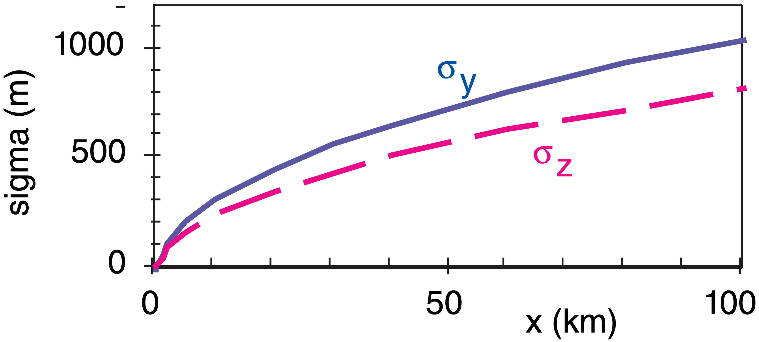
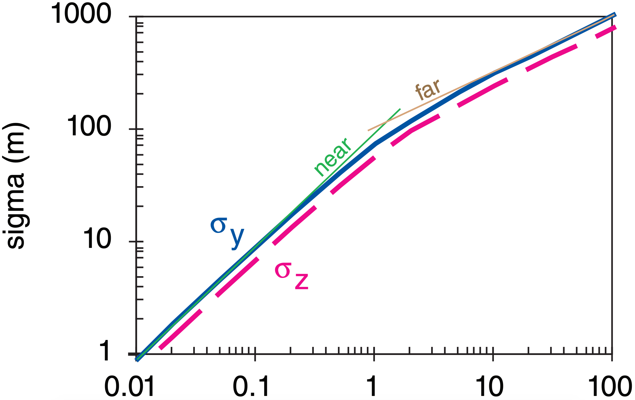
Plot vertical and horizontal plume spread σz and σy vs. downwind distance x, using a Lagrangian time scale of 1 minute and wind speed of 10 m s–1 at height 100 m in a neutral boundary layer of depth 500 m. There is a rough surface of varied crops.
a) Plot on both linear and log-log graphs. b) Also plot the short and long-distance limits of σy on the log-log graph.
Find the Answer
Given: z = 100 m, M = 10 m s–1, tL = 60 s, h = 500 m
Find: σz and σy (m) vs. x (km).
Refer to Atmospheric Boundary Layer chapter to calculate the info needed in the eqs. for Taylor’s statistical theory.
Use Table 18-1 for rough surface of varied crops: aerodynamic roughness length is zo = 0.25 m
Use this zo in eq. (18.13) to get the friction velocity: u* = [0.4·(10m s–1)] / ln(100m/0.25m) = 0.668 m s–1
Use this u* in eq. (18.25b) to get the velocity variance σv = 1.6·(0.668m s–1)·[1 – 0.5·(100m/500m)] = 0.96 m s–1 Similarly, use eq. (18.25c): σw = 0.75 m s–1.
Use σv and σw in eqs. (19.13a & b) in a spreadsheet to calculate σy and σz , and plot the results on graphs:

A linear graph is shown above, and log-log below.

Eqs. (19.14) & (19.15) for the near and far approximations are plotted as the thin solid lines.
Check: Units OK. Physics OK. Sketch OK.
Exposition: Plume spread increases with distance downwind of the smoke stack. σy ≈ σz at any x, giving the nearly isotropic dispersion expected for statically neutral air. The cross-over between short and long time limits is at x ≈ 2·M·tL = 1.2 km.


