19.4: Dispersion Statistics
- Page ID
- 9655
19.4.1. Snapshot vs. Average

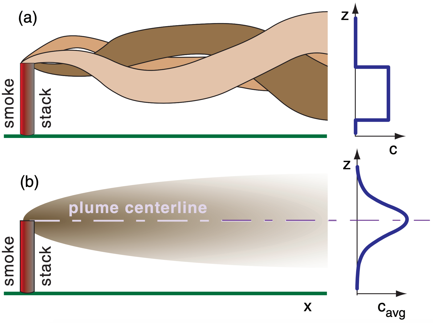
Snapshots of smoke plumes are similar to what you see with your eye. The plumes have fairly-well defined edges, but each plume wiggles up and down, left and right (Fig. 19.4a). The concentration c through such an instantaneous smoke plume can be quite variable, so a hypothetical vertical profile is sketched in Fig. 19.4a.
A time exposure of a smoke-stack plume might appear as sketched in Fig. 19.4b. When averaged over a time interval such as an hour, most of the pollutants are found near the centerline of the plume. Average concentration decreases smoothly with distance away from the centerline. The resulting profile of concentration is often bell shaped, or Gaussian. Air quality standards in most countries are based on averages, as was listed in Table 19–1.
19.4.2. Center of Mass
The plume centerline height zCL can be defined as the location of the center of mass of pollutants. In other words, it is the average height of the pollutants. Suppose you measure the concentration ck of pollutants at a range of equally-spaced heights zk through the smoke plume. The center of mass is a weighted average defined by:
\(\ \begin{align}z_{C L}=\bar{z}=\frac{\sum_{k=1}^{K} c_{k} \cdot z_{k}}{\sum_{k=1}^{K} c_{k}}\tag{19.8}\end{align}\)
where K is the total number of heights, k is the height index, and the overbar denotes a mean.
For passive tracers with slow exit velocity from the stack, the plume centerline is at the same height as the top of the stack. For buoyant plumes in hot exhaust gases, and for smoke blown at high speed out of the top of the stack, the centerline rises above the top of the stack.
A similar center of mass can be found for the crosswind (lateral) location, assuming measurements are made at equal intervals across the plume. Passive tracers blow downwind. Thus, the center of mass of a smoke plume, when viewed from above such as from a satellite, follows a mean wind trajectory from the stack location (see the discussion of streamlines, streaklines, and trajectories in the Regional Winds chapter).
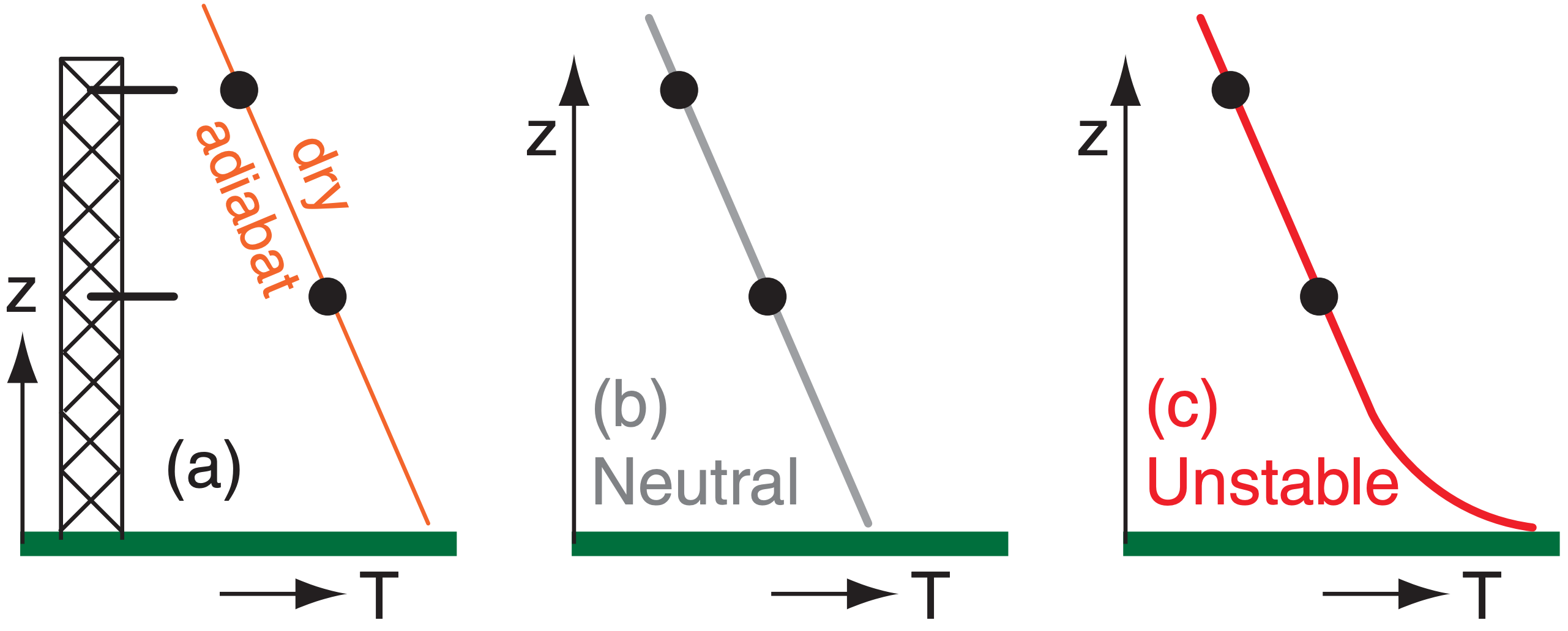
Incomplete data can be misinterpreted, leading to expensive erroneous conclusions. Suppose an air-pollution meteorologist/engineer erects a tall tower at the site of a proposed 75 m high smoke stack. On this tower are electronic thermometers at two heights: 50 and 100 m. On many days, these measurements give temperatures that are on the same adiabat (Fig. a).
Regarding static stability, one interpretation (Fig. b) is that the atmosphere is statically neutral. Another interpretation (Fig. c) is that it is a statically unstable convective mixed layer. If neutral stability is erroneously noted on a day of static instability, then the corresponding predictions of dispersion rate and concentrations will be embarrassingly wrong.
To resolve this dilemma, the meteorologist/engineer needs additional info. Either add a third thermometer near the ground, or add a net radiation sensor, or utilize manual observations of sun, clouds, and wind to better determine the static stability.

19.4.3. Standard Deviation – Sigma

For time-average plumes such as in Figs. 19.4b and 19.5, the plume edges are not easy to locate. They are poorly defined because the bell curve gradually approaches zero concentration with increasing distance from the centerline. Thus, we cannot use edges to measure plume spread (depth or width).
Instead, the standard deviation σz of pollutant location is used as a measure of plume spread, where standard deviation is the square root of the variance σz2 . The vertical-position deviations must be weighted by the pollution concentration to find sigma, as shown here:
\(\ \begin{align} \sigma_{z}=\left[\frac{\sum_{k=1}^{K} c_{k} \cdot\left(z_{k}-\bar{z}\right)^{2}}{\sum_{k=1}^{K} c_{k}}\right]^{1 / 2}\tag{19.9}\end{align}\)
where \(\ \bar{z}=z_{C L}\) is the average height found from the previous equation.
A similar equation can be defined for lateral standard deviation σy. The vertical and lateral dispersion need not be equal, because the dispersive nature of turbulence is not the same in the vertical and horizontal when turbulence is anisotropic.
When the plume is compact, the standard deviation and variance are small. These statistics increase as the plume spreads. Hence we expect sigma to increase with distance downwind of the stack. Such spread will be quantified in the next main section.
19.4.4. Gaussian Curve
The Gaussian or “normal” curve is bell shaped, and is given in one-dimension (1-D) by:
\(\ \begin{align}c(z)=\frac{Q_{1}}{\sigma_{z} \sqrt{2 \pi}} \cdot \exp \left\{-0.5\left[\frac{z-\bar{z}}{\sigma_{z}}\right]^{2}\right\}\tag{19.10}\end{align}\)
where c(z) is the one-dimensional concentration (g m–1) at any height z, and Q1 (g) is the total amount of pollutant emitted. Similar 1-D equations can be written for concentration in the x- or y-directions.
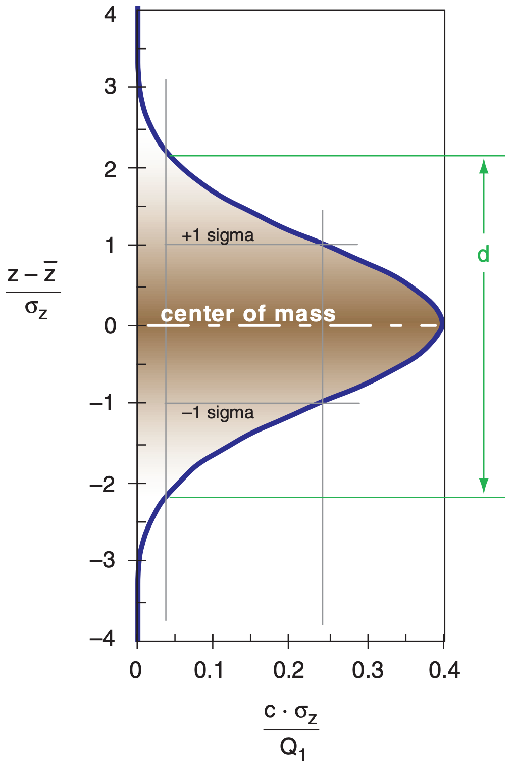
This curve is symmetric about the mean location, and has tails that asymptotically approach zero as z approaches infinity (Fig. 19.5). The area under the curve is equal to Q1, which physically means that pollutants are conserved. The inflection points in the curve (points where the curve changes from concave left to concave right) occur at exactly one σz from the mean. Between ±2·σz are 95% of the pollutants; hence, the Gaussian curve exhibits strong central tendency.
Eq. (19.10) has three parameters: Q1, \(\ \bar{z}\), and σz. These parameters can be estimated from measurements of concentration at equally-spaced heights through the plume, in order to find the best-fit Gaussian curve. The last two parameters are found with eqs. (19.8) and (19.9). The first parameter is found from:
\(\ \begin{align}Q_{1}=\Delta z \cdot \sum_{k=1}^{K} c_{k}\tag{19.11}\end{align}\)
where ∆z is the height interval between neighboring measurements.
Sample Application (§)
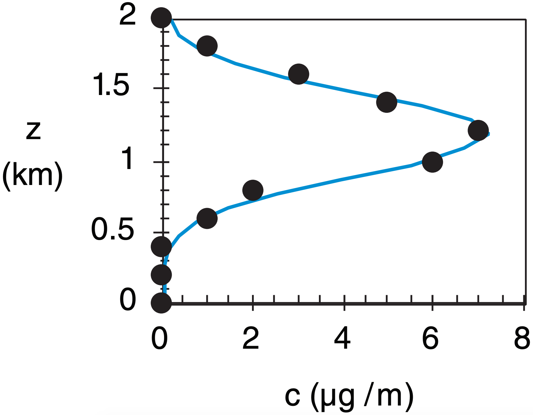
Given the following 1-D concentration measurements. Find the plume centerline height, standard deviation of height, and nominal plume depth. Plot the best-fit curve through these data points.
| z (km) | c(µg m–1) |
| 2.0 | 0 |
| 1.8 | 1 |
| 1.6 | 3 |
| 1.4 | 5 |
| 1.2 | 7 |
| 1.0 | 6 |
| 0.8 | 2 |
| 0.6 | 1 |
| 0.4 | 0 |
| 0.2 | 0 |
| 0.0 | 0 |
Find the Answer
Given: ∆z = 0.2 km, with concentrations above
Find:\(\ \bar{z}\) = ? km, σz = ? km, Q1 = ? km·µg m–1, d = ? km, and plot c(z) = ? µg m–1
Use eq. (19.8) to find the plume centerline height:
\(\ \bar{z} \) = (30.2 km·µg·m–1) / (25 µg·m–1) = 1.208 km
Use eq. (19.9):
σz2 = (1.9575 km2·µg·m–1)/(25 µg·m–1) = 0.0783 km2
σz = [ σz2 ]1/2 = [0.0783 km2 ]1/2 = 0.28 km
Use eq. (19.12):
d = 4.3 · (0.28 km) = 1.2 km
Use eq. (19.11):
Q1 = (0.2 km) · (25 µg·m–1) = 5.0 km·µg m–1
Use eq. (19.10) to plot the best-fit curve:

Check: Units OK. Physics OK. Sketch OK.
Exposition: The curve is a good fit to the data. Often the measured data will have some scatter due to the difficulty of making concentration measurements, but the equations in this section are able to find the bestfit curve. This statistical curve-fitting method is called the method of moments, because we matched the first two statistical moments (mean & variance) of the Gaussian distribution to the corresponding moments calculated from the data.
19.4.5. Nominal Plume Edge
For practical purposes, the edge of a Gaussian plume is defined as the location where the concentration is 10% of the centerline concentration. This gives a plume spread (e.g., depth from top edge to bottom edge) of
\(\ \begin{align}d \approx 4.3 \cdot \sigma_{z}\tag{19.12}\end{align}\)


