
3.8.3: Kelvin waves
- Page ID
- 16308

\( \newcommand{\vecs}[1]{\overset { \scriptstyle \rightharpoonup} {\mathbf{#1}} } \)
\( \newcommand{\vecd}[1]{\overset{-\!-\!\rightharpoonup}{\vphantom{a}\smash {#1}}} \)
\( \newcommand{\dsum}{\displaystyle\sum\limits} \)
\( \newcommand{\dint}{\displaystyle\int\limits} \)
\( \newcommand{\dlim}{\displaystyle\lim\limits} \)
\( \newcommand{\id}{\mathrm{id}}\) \( \newcommand{\Span}{\mathrm{span}}\)
( \newcommand{\kernel}{\mathrm{null}\,}\) \( \newcommand{\range}{\mathrm{range}\,}\)
\( \newcommand{\RealPart}{\mathrm{Re}}\) \( \newcommand{\ImaginaryPart}{\mathrm{Im}}\)
\( \newcommand{\Argument}{\mathrm{Arg}}\) \( \newcommand{\norm}[1]{\| #1 \|}\)
\( \newcommand{\inner}[2]{\langle #1, #2 \rangle}\)
\( \newcommand{\Span}{\mathrm{span}}\)
\( \newcommand{\id}{\mathrm{id}}\)
\( \newcommand{\Span}{\mathrm{span}}\)
\( \newcommand{\kernel}{\mathrm{null}\,}\)
\( \newcommand{\range}{\mathrm{range}\,}\)
\( \newcommand{\RealPart}{\mathrm{Re}}\)
\( \newcommand{\ImaginaryPart}{\mathrm{Im}}\)
\( \newcommand{\Argument}{\mathrm{Arg}}\)
\( \newcommand{\norm}[1]{\| #1 \|}\)
\( \newcommand{\inner}[2]{\langle #1, #2 \rangle}\)
\( \newcommand{\Span}{\mathrm{span}}\) \( \newcommand{\AA}{\unicode[.8,0]{x212B}}\)
\( \newcommand{\vectorA}[1]{\vec{#1}} % arrow\)
\( \newcommand{\vectorAt}[1]{\vec{\text{#1}}} % arrow\)
\( \newcommand{\vectorB}[1]{\overset { \scriptstyle \rightharpoonup} {\mathbf{#1}} } \)
\( \newcommand{\vectorC}[1]{\textbf{#1}} \)
\( \newcommand{\vectorD}[1]{\overrightarrow{#1}} \)
\( \newcommand{\vectorDt}[1]{\overrightarrow{\text{#1}}} \)
\( \newcommand{\vectE}[1]{\overset{-\!-\!\rightharpoonup}{\vphantom{a}\smash{\mathbf {#1}}}} \)
\( \newcommand{\vecs}[1]{\overset { \scriptstyle \rightharpoonup} {\mathbf{#1}} } \)
\( \newcommand{\vecd}[1]{\overset{-\!-\!\rightharpoonup}{\vphantom{a}\smash {#1}}} \)
\(\newcommand{\avec}{\mathbf a}\) \(\newcommand{\bvec}{\mathbf b}\) \(\newcommand{\cvec}{\mathbf c}\) \(\newcommand{\dvec}{\mathbf d}\) \(\newcommand{\dtil}{\widetilde{\mathbf d}}\) \(\newcommand{\evec}{\mathbf e}\) \(\newcommand{\fvec}{\mathbf f}\) \(\newcommand{\nvec}{\mathbf n}\) \(\newcommand{\pvec}{\mathbf p}\) \(\newcommand{\qvec}{\mathbf q}\) \(\newcommand{\svec}{\mathbf s}\) \(\newcommand{\tvec}{\mathbf t}\) \(\newcommand{\uvec}{\mathbf u}\) \(\newcommand{\vvec}{\mathbf v}\) \(\newcommand{\wvec}{\mathbf w}\) \(\newcommand{\xvec}{\mathbf x}\) \(\newcommand{\yvec}{\mathbf y}\) \(\newcommand{\zvec}{\mathbf z}\) \(\newcommand{\rvec}{\mathbf r}\) \(\newcommand{\mvec}{\mathbf m}\) \(\newcommand{\zerovec}{\mathbf 0}\) \(\newcommand{\onevec}{\mathbf 1}\) \(\newcommand{\real}{\mathbb R}\) \(\newcommand{\twovec}[2]{\left[\begin{array}{r}#1 \\ #2 \end{array}\right]}\) \(\newcommand{\ctwovec}[2]{\left[\begin{array}{c}#1 \\ #2 \end{array}\right]}\) \(\newcommand{\threevec}[3]{\left[\begin{array}{r}#1 \\ #2 \\ #3 \end{array}\right]}\) \(\newcommand{\cthreevec}[3]{\left[\begin{array}{c}#1 \\ #2 \\ #3 \end{array}\right]}\) \(\newcommand{\fourvec}[4]{\left[\begin{array}{r}#1 \\ #2 \\ #3 \\ #4 \end{array}\right]}\) \(\newcommand{\cfourvec}[4]{\left[\begin{array}{c}#1 \\ #2 \\ #3 \\ #4 \end{array}\right]}\) \(\newcommand{\fivevec}[5]{\left[\begin{array}{r}#1 \\ #2 \\ #3 \\ #4 \\ #5 \\ \end{array}\right]}\) \(\newcommand{\cfivevec}[5]{\left[\begin{array}{c}#1 \\ #2 \\ #3 \\ #4 \\ #5 \\ \end{array}\right]}\) \(\newcommand{\mattwo}[4]{\left[\begin{array}{rr}#1 \amp #2 \\ #3 \amp #4 \\ \end{array}\right]}\) \(\newcommand{\laspan}[1]{\text{Span}\{#1\}}\) \(\newcommand{\bcal}{\cal B}\) \(\newcommand{\ccal}{\cal C}\) \(\newcommand{\scal}{\cal S}\) \(\newcommand{\wcal}{\cal W}\) \(\newcommand{\ecal}{\cal E}\) \(\newcommand{\coords}[2]{\left\{#1\right\}_{#2}}\) \(\newcommand{\gray}[1]{\color{gray}{#1}}\) \(\newcommand{\lgray}[1]{\color{lightgray}{#1}}\) \(\newcommand{\rank}{\operatorname{rank}}\) \(\newcommand{\row}{\text{Row}}\) \(\newcommand{\col}{\text{Col}}\) \(\renewcommand{\row}{\text{Row}}\) \(\newcommand{\nul}{\text{Nul}}\) \(\newcommand{\var}{\text{Var}}\) \(\newcommand{\corr}{\text{corr}}\) \(\newcommand{\len}[1]{\left|#1\right|}\) \(\newcommand{\bbar}{\overline{\bvec}}\) \(\newcommand{\bhat}{\widehat{\bvec}}\) \(\newcommand{\bperp}{\bvec^\perp}\) \(\newcommand{\xhat}{\widehat{\xvec}}\) \(\newcommand{\vhat}{\widehat{\vvec}}\) \(\newcommand{\uhat}{\widehat{\uvec}}\) \(\newcommand{\what}{\widehat{\wvec}}\) \(\newcommand{\Sighat}{\widehat{\Sigma}}\) \(\newcommand{\lt}{<}\) \(\newcommand{\gt}{>}\) \(\newcommand{\amp}{&}\) \(\definecolor{fillinmathshade}{gray}{0.9}\)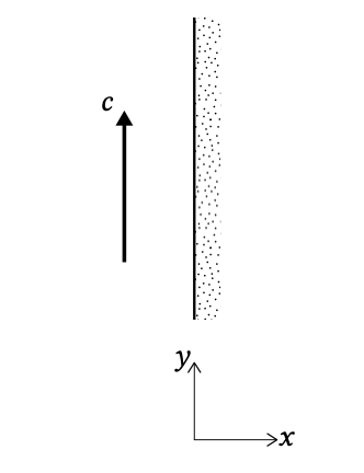
As coastal engineers we are interested in the tidal propagation and the tidal range along the boundaries of oceans and seas. To understand more about the propagation along closed coastal boundaries we need a further understanding of the rotary wave forming the amphidromic system. These waves depend on the existence of a closed boundary. A definition sketch is given in Fig. 3.32. Wave propagation is in the positive \(y\)-direction in the Northern Hemisphere (NH), hence \(c\) is positive. Such a wave would deflect from this eastern boundary in the Southern Hemisphere (SH) because of Coriolis. Therefore, for the SH we expect a wave propagating in the negative \(y\)-direction (\(c\) negative).
As before, we assume a more or less horizontal bottom slope and a small tidal amplitude compared to the water depth. Balancing inertia, Coriolis, the pressure gradient and bed friction leads to the following reduced shallow water equations in two horizontal dimensions:
\[\dfrac{\partial u}{\partial t} - fv = -g \dfrac{\partial \eta}{\partial x} - \dfrac{\tau_{b,x}}{\rho h}\label{eq3.8.3.1}\]
\[\dfrac{\partial v}{\partial t} + fu = -g \dfrac{\partial \eta}{\partial y} - \dfrac{\tau_{b,y}}{\rho h}\label{eq3.8.3.2}\]
where
| \(u, v\) | velocity in \(x,y\)-direction | \(m/s\) |
| \(f\) | \(2 \omega_e \sin \varphi\) is the Coriolis parameter with the earth's angular velocity \(\omega_e = 72.9 \times 10^{-6}\ rad/s\) and the latitude \(\varphi\) positive in the NH and negative in the SH | \(1/s\) |
| \(\eta\) | oscillatory water level variation | \(m\) |
| \(\tau_{b, x}\) | bottom shear stress in \(x\) direction | \(N/m^2\) |
| \(\tau_{b, y}\) | bottom shear stress in \(x\) direction | \(N/m^2\) |
| \(\rho\) | water density | \(kg/m^3\) |
| \(h\) | water depth | \(m\) |
The Coriolis acceleration has been introduced in the above equations of motion in such a way that it makes a right angle with the particle velocity and acts towards the right (to starboard side) in the NH and towards the left (to port) in the SH (see Intermezzo 3.1). Check for yourself the signs of the Coriolis terms in Eqs. \(\ref{eq3.8.3.1}\) and \(\ref{eq3.8.3.2}\). In doing so, note that the latitude \(\varphi\) and hence the Coriolis parameter \(f\) are assumed to have positive values in the NH and negative values in the SH.
Continuity requires:
\[\dfrac{\partial \eta}{\partial t} + h \left (\dfrac{\partial u}{\partial x} + \dfrac{\partial v}{\partial y} \right ) = 0\]
If we neglect friction and realise that the velocity \(u\) at the closed boundary (the coast- line) is zero the balance equations reduce to:
\[-fv = -g \dfrac{\partial \eta}{\partial x}\label{eq3.8.3.3}\]
\[\dfrac{\partial v}{\partial t} = -g \dfrac{\partial \eta }{\partial y} \label{eq3.8.3.4}\]
\[h \dfrac{\partial v}{\partial y} = -\dfrac{\partial \eta}{\partial t}\label{eq3.8.3.5}\]
Notice that the cross-shore (\(x\)) momentum balance (Eq. \(\ref{eq3.8.3.3}\)) is geostrophic: there is a balance between Coriolis force and the pressure gradient due to water level differences. This is comparable to the influence of Coriolis on the flow in a confined channel (see Intermezzo 3.6). The alongshore momentum balance, Eq. \(\ref{eq3.8.3.4}\), is the same as that for shallow water gravity waves (the progressive tidal waves from Intermezzo 3.5). Equation \(\ref{eq3.8.3.4}\) combined with the reduced continuity equation, Eq. \(\ref{eq3.8.3.5}\) yields a set of equations that it equivalent to Eqs. 3.8.1.2 and 3.8.1.3 and thus has an equivalent solution. Now substitute this solution \(\eta = \hat{\eta} \cos (\omega t - ky)\) and \(v = g/c \eta\) with \(c = \pm \sqrt{gh}\) in the geostrophic flow equation, Eq. \(\ref{eq3.8.3.3}\). The resulting equation now gives a solution known as a Kelvin wave:
\[\eta (x, y, t) = \eta_0 e^{(\tfrac{fx}{c})} \cos (\omega t - ky)\]
\[v(x, y, t) = \tfrac{c}{h} \eta_0 e^{(\tfrac{fx}{c})} \cos (\omega t - ky)\]
The Kelvin wave propagates along the coast (in the \(y\)-direction) at the shallow water speed. The alongshore velocity is in phase with the water level (as for the propagating wave of Intermezzo 3.5). The amplitude is maximum at the coast (\(\eta_0\)) and then decays with distance from the coast (in the negative \(x\)-direction). The scale of the decay is \(c/f\) in which the variables are the latitude and the water depth:
\[\dfrac{c}{f} = \sqrt{gh} \dfrac{1}{1.46 \times 10^{-4} \times \sin \varphi} = 21453 \dfrac{\sqrt{h}}{\sin \varphi}\]
At 45° latitude this amounts to about 1900 km for the deep oceans with an average water depth of 4000 m and to a good 200 km for a shallow sea with a typical water depth of 50 m.
The value of \(c/f\) cannot be negative, since this would make the sea level grow exponentially offshore. This implies, as expected, that the Kelvin wave propagates in the positive \(y\)-direction in the NH (where \(f\) is positive) and in the negative \(y\)-direction in the SH (where \(f\) is negative).
If the flow takes place in a confined conduit or channel that prevents a deviation of the course (i.e. a steady current), the Coriolis acceleration causes a pressure gradient across the conduit:
\[\dfrac{1}{\rho} \dfrac{\partial p}{\partial n} = 2 \omega_e V \sin \varphi\]
where
| \(\rho\) | water density | \(kg/m^3\) |
| \(\rho\) | water pressure | \(N/m^2\) |
| \(n\) | normal to and directed to starboard of the current \(V\) | - |
In open channel flow, the pressure gradient becomes visible as a gradient of the water surface:
\[\dfrac{1}{\rho} \dfrac{\partial p}{\partial n} = g \dfrac{\partial \eta}{\partial n}\]
Note: upon comparing the above two equations (Eqs. 3.45 and 3.46) with the full depth-integrated shallow water equations it can be seen that only the pressure gradient due to the water level surface and the Coriolis acceleration are retained.
As an example, we compute the sea level difference across the Strait of Florida. The Florida Current is located at latitude 26°N; the current velocity is about 1 m/s; the width of the Strait of Florida is about 80 km.
\[\dfrac{1}{\rho} \dfrac{\partial p}{\partial n} = 2 \cdot 0.729 \times 10^4 \cdot \sin 26^{\circ} \cdot 1 = 6.4 \times 10^{-5} m/s^2\]
The elevation difference over 80 km is computed as follows:
\[\Delta \eta = \dfrac{1}{\rho} \dfrac{\partial p}{\partial n} \dfrac{\Delta x}{g} = \dfrac{6.4 \times 10^{-5}}{9.81} \cdot 80 \times 10^3 = 0.52m\]
The observed value is 0.45 m, which is close to our estimate. (Similar computations can be made for e.g. the Western Scheldt, the British Channel or the Dutch Texel Inlet).
The Kelvin wave is a coastally trapped wave; it needs a coastline. In the NH, the wave propagates poleward along an eastern boundary and equatorward along a western boundary with its maximum amplitude at the boundary. It thus forms a wave trapped to the boundary and rotating counter-clockwise around an amphidromic point (like a standing wave, but now rotating). The rotation is clockwise in the SH.
In the North Sea multiple amphidromic points can be observed (see Fig. 3.31). The Kelvin wave enters the North Sea basin from the north. Some of the energy is dissipated in the basin and some is reflected from the shallow areas in the southern part of the North Sea. This reflected wave forms its own amphidromic system.
For the ideal Kelvin wave, friction is not taken into account. Neglecting friction can be a good approximation for deeper water. Near the coast inertia is relatively unimportant but bottom friction needs to be taken into account. The velocity is then governed by the balance between the bottom friction and the alongshore water level gradient. This will be treated in more detail in Ch. 5.