

18: Atmospheric Boundary Layer
- Page ID
- 9651
\( \newcommand{\vecs}[1]{\overset { \scriptstyle \rightharpoonup} {\mathbf{#1}} } \)
\( \newcommand{\vecd}[1]{\overset{-\!-\!\rightharpoonup}{\vphantom{a}\smash {#1}}} \)
\( \newcommand{\dsum}{\displaystyle\sum\limits} \)
\( \newcommand{\dint}{\displaystyle\int\limits} \)
\( \newcommand{\dlim}{\displaystyle\lim\limits} \)
\( \newcommand{\id}{\mathrm{id}}\) \( \newcommand{\Span}{\mathrm{span}}\)
( \newcommand{\kernel}{\mathrm{null}\,}\) \( \newcommand{\range}{\mathrm{range}\,}\)
\( \newcommand{\RealPart}{\mathrm{Re}}\) \( \newcommand{\ImaginaryPart}{\mathrm{Im}}\)
\( \newcommand{\Argument}{\mathrm{Arg}}\) \( \newcommand{\norm}[1]{\| #1 \|}\)
\( \newcommand{\inner}[2]{\langle #1, #2 \rangle}\)
\( \newcommand{\Span}{\mathrm{span}}\)
\( \newcommand{\id}{\mathrm{id}}\)
\( \newcommand{\Span}{\mathrm{span}}\)
\( \newcommand{\kernel}{\mathrm{null}\,}\)
\( \newcommand{\range}{\mathrm{range}\,}\)
\( \newcommand{\RealPart}{\mathrm{Re}}\)
\( \newcommand{\ImaginaryPart}{\mathrm{Im}}\)
\( \newcommand{\Argument}{\mathrm{Arg}}\)
\( \newcommand{\norm}[1]{\| #1 \|}\)
\( \newcommand{\inner}[2]{\langle #1, #2 \rangle}\)
\( \newcommand{\Span}{\mathrm{span}}\) \( \newcommand{\AA}{\unicode[.8,0]{x212B}}\)
\( \newcommand{\vectorA}[1]{\vec{#1}} % arrow\)
\( \newcommand{\vectorAt}[1]{\vec{\text{#1}}} % arrow\)
\( \newcommand{\vectorB}[1]{\overset { \scriptstyle \rightharpoonup} {\mathbf{#1}} } \)
\( \newcommand{\vectorC}[1]{\textbf{#1}} \)
\( \newcommand{\vectorD}[1]{\overrightarrow{#1}} \)
\( \newcommand{\vectorDt}[1]{\overrightarrow{\text{#1}}} \)
\( \newcommand{\vectE}[1]{\overset{-\!-\!\rightharpoonup}{\vphantom{a}\smash{\mathbf {#1}}}} \)
\( \newcommand{\vecs}[1]{\overset { \scriptstyle \rightharpoonup} {\mathbf{#1}} } \)
\(\newcommand{\longvect}{\overrightarrow}\)
\( \newcommand{\vecd}[1]{\overset{-\!-\!\rightharpoonup}{\vphantom{a}\smash {#1}}} \)
\(\newcommand{\ket}[1]{\left| #1 \right>}\)
\(\newcommand{\bra}[1]{\left< #1 \right|}\)
\(\newcommand{\braket}[2]{\left< #1 \vphantom{#2} \right| \left. #2 \vphantom{#1} \right>}\)
\(\newcommand{\braopket}[3]{\left< #1 \vphantom{#2}\vphantom{#3} \right| #2 \vphantom{#1}\vphantom{#3} \left| #3 \vphantom{#1}\vphantom{#2} \right>}\)
\(\newcommand{\qmvec}[1]{\mathbf{\vec{#1}}}\)
\(\newcommand{\op}[1]{\hat{\mathbf{#1}}}\)
\(\newcommand{\expect}[1]{\langle #1 \rangle}\)
\(\newcommand{\dfn}[1]{\emph{\textbf{#1}}}\)
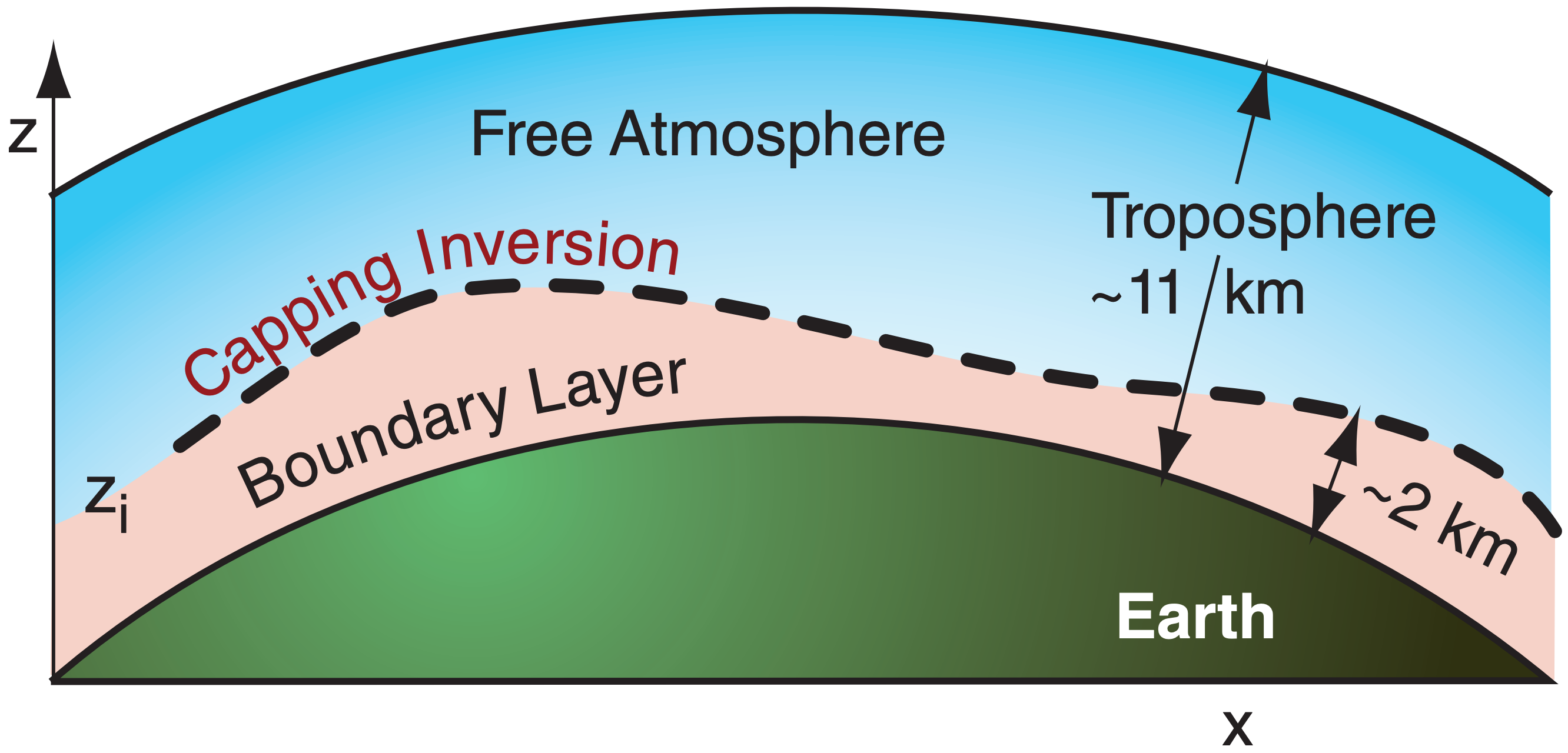
Sunrise, sunset, sunrise. The daily cycle of radiative heating and cooling of the Earth’s surface during clear skies causes a daily cycle of sensible and latent heat fluxes between the land and the air. These fluxes modify the bottom of the troposphere — a layer called the atmospheric boundary layer (ABL) because it is influenced by the bottom boundary of the atmosphere (Fig. 18.1).
The ABL experiences a diurnal (daily) cycle of temperature, humidity, wind, and pollution variations in response to the varying surface fluxes. Turbulence is ubiquitous in the ABL, and is one of the causes of the unique nature of the ABL.
Because the boundary layer is where we live, where our crops are grown, and where we conduct our commerce, we have become familiar with its daily cycle. We perhaps forget that this cycle is not experienced by the rest of the atmosphere above the ABL. This chapter examines the formation and unique characteristics of the ABL.
- 18.1: Static Stability - a Review
- This page discusses the Atmospheric Boundary Layer (ABL), detailing its depth and how temperature inversions create a stable atmosphere that affects wind, temperature profiles, and turbulence, restricting vertical motion. It highlights the implications of these inversions on pollution and weather patterns, influenced by surface heating and synoptic systems.
- 18.3: ABL Structure and Evolution
- This page outlines the atmospheric boundary layer (ABL) components during summer fair weather over land, highlighting the differences between the daytime statically unstable mixed layer (ML) and nighttime statically stable boundary layer (SBL) beneath a neutral residual layer (RL).
- 18.4: Temperature
- This page covers the Atmospheric Boundary Layer (ABL), detailing how cumulative heating and cooling affect its dynamics. It explains daytime heating leading to turbulence and nighttime cooling resulting in stability, influenced by seasonal variations. Techniques for estimating temperature profiles and mixed-layer growth using the encroachment method and focusing on entrainment dynamics are discussed.
- 18.5: Wind
- This page examines the dynamics of wind speeds in the Atmospheric Boundary Layer (ABL), highlighting factors such as friction, surface roughness, and turbulence. It explores subgeostrophic conditions, diurnal wind profile variations, and the impact of surface roughness on drag coefficients and friction velocity. Additionally, it details wind speed profiles in stable and unstable ABLs, utilizing specific calculations to demonstrate uniform wind speed transitions at greater altitudes.
- 18.6: Turbulence
- This page covers key aspects of wind speed, turbulence, and their implications for meteorology, including mean wind, turbulence characteristics in the atmospheric boundary layer, and turbulent kinetic energy (TKE) dynamics. It discusses how turbulence is influenced by stability, shear, and buoyancy, along with statistical measurements like variances and fluxes.
- 18.7: Review
- This page discusses the atmospheric boundary layer (ABL), which ranges from 200 m to 4 km and shows daily variations due to solar effects. Turbulence during the day mixes atmospheric variables, leading to a uniform layer, while at night, a stable layer with weak turbulence develops. Surface drag affects wind profiles in the surface layer.
- 18.8: Homework Exercises
- This page covers exercises to enhance understanding of atmospheric boundary layers (ABL) using rawinsonde data, examining wind speed, turbulence, and heat flux dynamics. It highlights calculation techniques for wind and temperature effects under varied conditions and explores ABL characteristics during different weather phenomena.