14.3: High Humidity in the ABL

One of the four conditions needed to form convective storms such as thunderstorms is high humidity in the atmospheric boundary layer (ABL). Thunderstorms draw in pre-storm ABL air, which rises and cools in the thunderstorm updraft. As water vapor condenses, it releases latent heat, which is the main energy source for the storm (see the Sample Application). Thus, the ABL is the fuel tank for the storm. In general, stronger thunderstorms form in moister warmer ABL air (assuming all other factors are constant, such as the environmental sounding, wind shear, trigger, etc.).

The dew-point temperature T_d in the ABL is a good measure of the low-altitude humidity. High dew points also imply high air temperature, because T ≥ T_d always (see the Water Vapor chapter). Higher temperatures indicate more sensible heat, and higher humidity indicates more latent heat. Thus, high dew points in the ABL indicate a large fuel supply in the ABL environment that can be tapped by thunderstorms. Thunderstorms in regions with T_d ≥ 16°C can have heavy precipitation, and those in regions with T_d ≥ 21°C can have greater severity.

Figure 14.28 Surface weather map valid at 22 UTC on 24 May 2006 showing isodrosotherms (lines of equal dew-point, T_d, in °C) over N. America. Moistest air is shaded, and highlights the greatest fuel supply for thunderstorms. A dry line (sharp decrease in humidity) exists in west Texas (TX) and Oklahoma (OK).

Note, this is a different case study than was used in the previous chapter. The Extratropical Cyclone chapter used a Winter storm case, while here we use an early Spring severe-storm case.

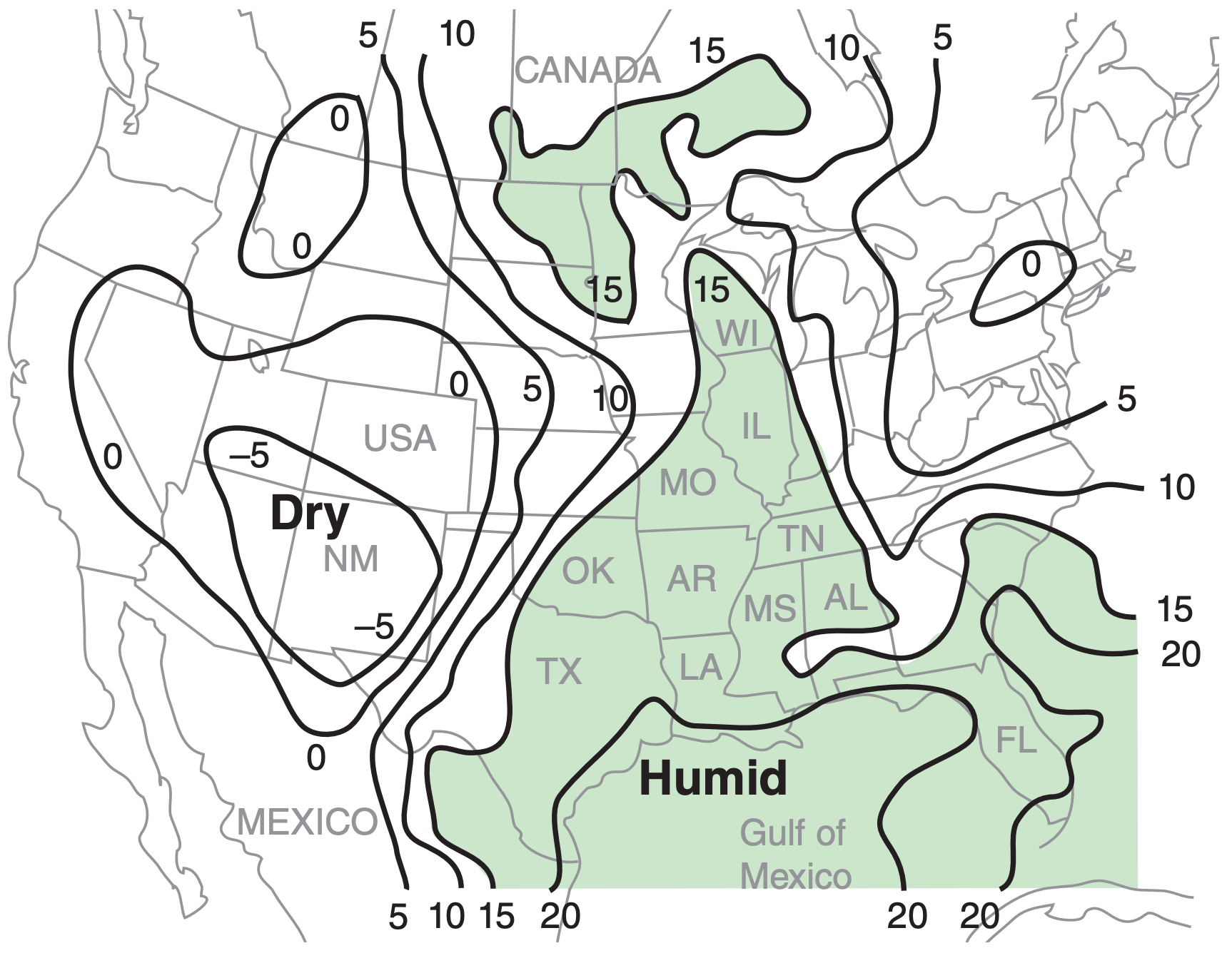
On weather maps, lines of equal dew-point temperature are called isodrosotherms (recall Table 1-6). Fig. 14.28 shows an example, where the isodrosotherms are useful for identifying regions having warm humid boundary layers.

Most of the weather maps in this chapter and the next chapter are from a severe weather case on 24 May 2006. These case-study maps are meant to give one example, and do not show average or climatological conditions. The actual severe weather that occurred for this case is described at the end of this chapter, just before the Review.

An alternative moisture variable is mixing ratio, r. Large mixing-ratio values are possible only if the air is warm (because warm air can hold more water vapor at saturation), and indicate greater energy available for thunderstorms. For example, Fig. 14.29 shows isohumes of mixing ratio.

Wet-bulb temperature T_w , wet-bulb potential temperature θ_w , equivalent potential temperature θ_e , or liquid-water potential temperature θ_L also indicate moisture. Recall from Normand’s rule in the Water Vapor chapter that the wet-bulb potential temperature corresponds to the moist adiabat that passes through the LCL on a thermo diagram. Also in the Water-Vapor chapter is a graph relating θ_w to θ_e.

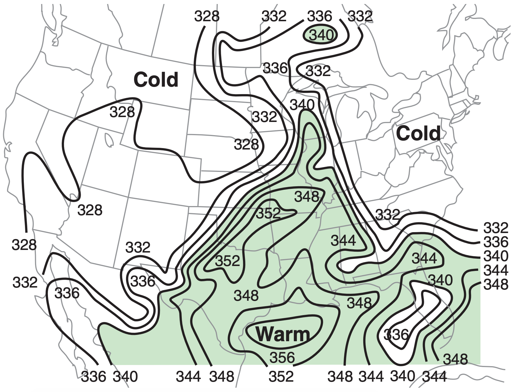
For afternoon thunderstorms in the USA, prestorm boundary layers most frequently have wetbulb potential temperatures in the θ_w = 20 to 28°C range (or θ_e in the 334 to 372 K range, see example in Fig. 14.30). For supercell thunderstorms, the boundary-layer average is about θ_w = 24°C (or θ_e = 351 K), with some particularly severe storms (strong tornadoes or large hail) having θ_w ≥ 27°C (or θ_e ≥ 366 K).

Figure 14.29 Similar to the previous weather map, but for isohumes of mixing ratio (g·kg^–1).

Figure 14.30 Similar to previous figure, but for equivalent potential temperature θ_e in Kelvin. Larger θ_e indicates warmer, moister air.

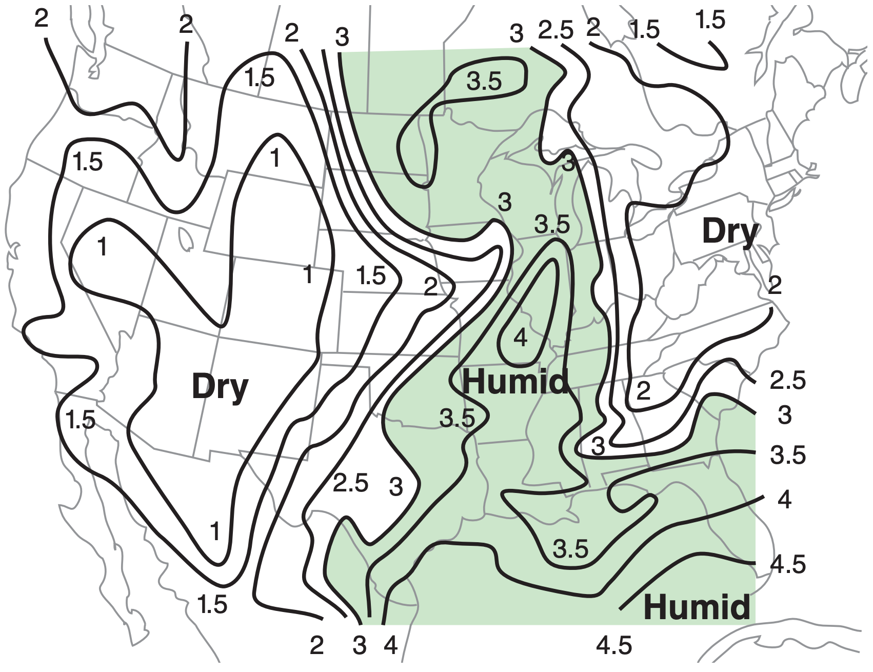
Precipitable water gives the total water content in a column of air from the ground to the top of the atmosphere (see example in Fig. 14.31). It does not account for additional water advected into the storm by the inflow winds, and thus is not a good measure of the total amount of water vapor that can condense and release energy.

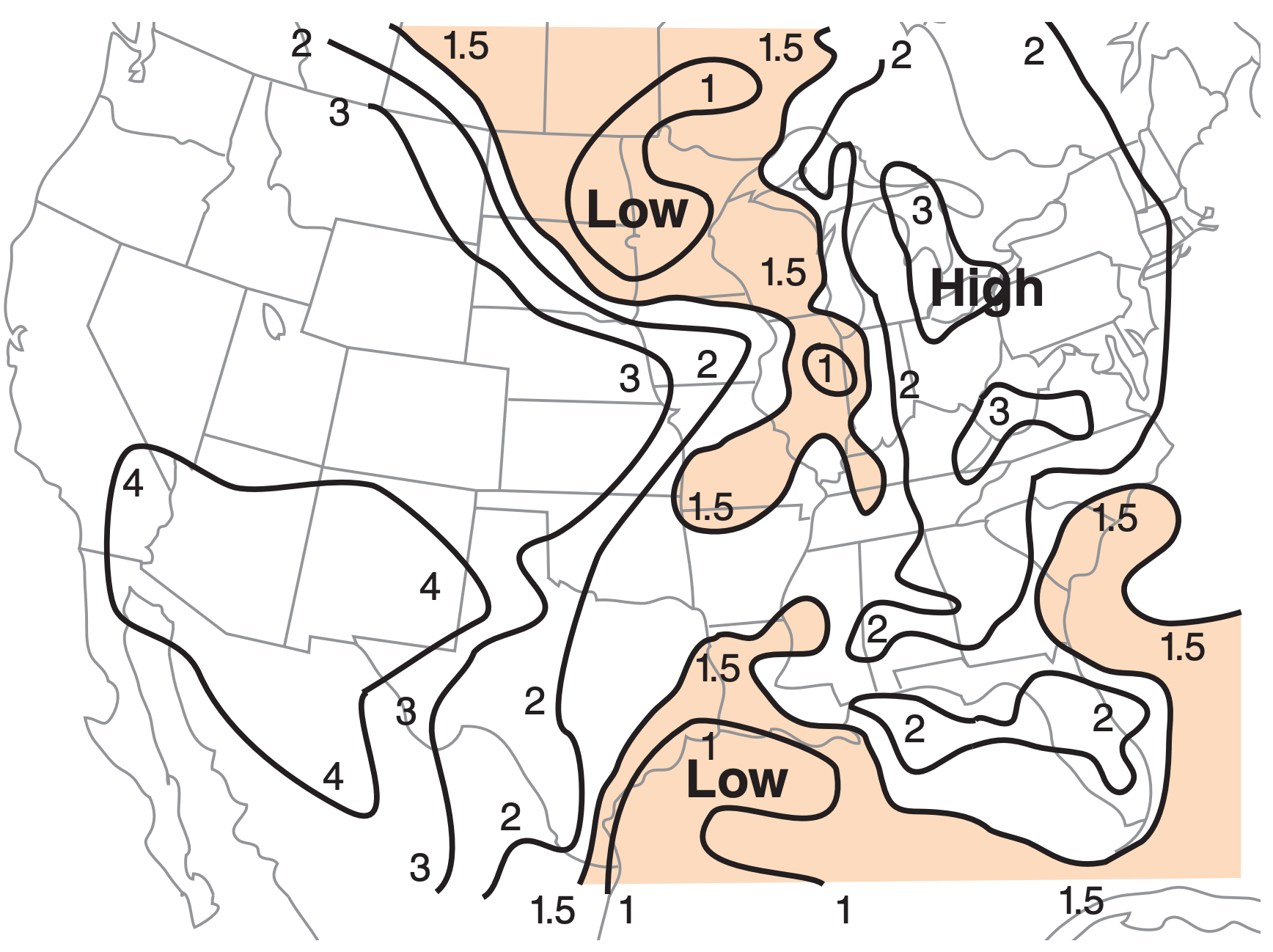
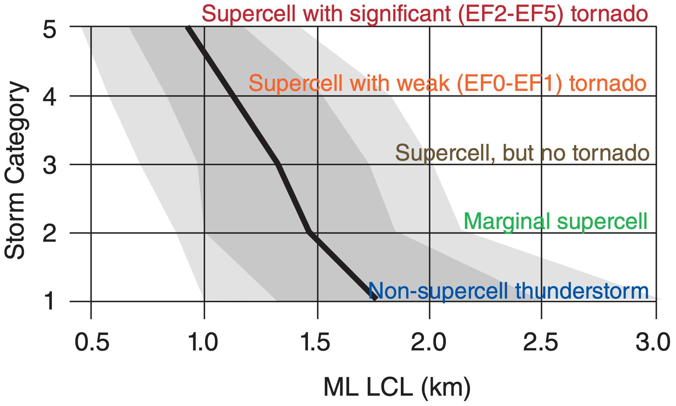
Mean-layer lifting condensation level (MLLCL) is the average of the LCL altitudes for all air parcels starting at heights within the bottom 1 km of the atmosphere (i.e., ≈ boundary layer). Lower MLLCL values indicate greater ABL moisture, and favor stronger storms (Figs. 14.32 & 14.33).

Figure 14.31 Similar to previous figure, but for precipitable water in cm.

Figure 14.32 Similar to previous figure, but for mean-layer lifting condensation level (ML-LCL) heights in km above ground level. Lower ML-LCL heights (suggesting more intense storms) are shaded.

Figure 14.33 Statistical relationship between storm category (as labeled along the horizontal lines) and the mean-layer lifting condensation level (ML-LCL). A marginal supercell is one with weak (< 20 m s^–1) or short-duration (< 30 min) cyclonic shear. EF is the Enhanced Fujita scale tornado intensity. Thick line is median (50 percentile) of about 500 observed thunderstorms in the central USA. Dark grey spans 25th through 75th percentiles (i.e., the interquartile range), and light grey spans 10th through 90th percentiles. Lower ML-LCL values generally correspond to greater storm intensities. Caution: There is significant overlap of ML-LCLs for all storm categories, implying that ML-LCL cannot sharply discriminate between storm severities.

See the INFO box on the next page to learn about the median, interquartile range, and percentiles.

INFO • Median, Quartiles, Percentiles

Median, quartiles, and percentiles are statistical ways to summarize the location and spread of experimental data. They are a robust form of data reduction, where hundreds or thousands of data are represented by several summary statistics.

First, sort your data from the smallest to largest values. This is easy to do on a computer. Each data point now has a rank associated with it, such as 1^st (smallest value), 2^nd, 3^rd, ... n^th (largest value). Let x(r) = the value of the rth ranked data point.

The middle-ranked data point [i.e., at r = (1/2)·(n+1)] is called the median, and the data value x of this middle data point is the median value (q_0.5). Namely,

q_0.5 = x_(1/2)·(n+1) for n = odd

If n is an even number, there is no data point exactly in the middle, so use the average of the 2 closest points:

q_0.5 = 0.5· [x_(n/2) + x_(n/2)+1 ] for n = even

The median is a measure of the location or center of the data

The data point with a rank closest to r = (1/4)·(n+1) is the lower quartile point:

q_0.25 = x_(1/4)·(n+1)

The data point with a rank closest to r = (3/4)·(n+1) is the upper quartile point:

q_0.75 = x_(3/4)·(n+1)

These last 2 equations work well if n is large (≥100, see below). The interquartile range (IQR) is defined as IQR = q_0.75 – q_0.25 , and is a measure of the spread of the data. (See the Sample Application nearby.)

Generically, the variable q_p represents any quantile, namely the value of the ranked data point having a value that exceeds portion p of all data points. We already looked at p = 1/4, 1/2, and 3/4. We could also divide large data sets into hundredths, giving percentiles. The lower quartile is the same as the 25th percentile, the median is the 50th percentile, and the upper quartile is the 75^th percentile.

These non-parametric statistics are robust (usually give a reasonable answer regardless of the actual distribution of data) and resistant (are not overly influenced by outlier data points). For comparison, the mean and standard deviation are NOT robust nor resistant. Thus, for experimental data, you should use the median and IQR.

To find quartiles for a small data set, split the ranked data in half, and look at the lower and upper halves separately.

Lower half of data: If n = odd, consider the data points ranked less than or equal to the median point. For n = even, consider points with values less than the median value. For this subset of data, find its median, using the same tricks as in the previous paragraph. The resulting data point is the lower quartile.

Upper half of data: For n = odd, consider the data points ranked greater than or equal to the original median point. For n = even, use the points with values greater than the median value. The median point in this data subset gives the upper quartile.

Sample Application (§)

Suppose the z_LCL (km) values for 9 supercells (with EF0-EF1 tornadoes) are:

1.5, 0.8, 1.4, 1.8, 8.2, 1.0, 0.7, 0.5, 1.2

Find the median and interquartile range. Compare with the mean and standard deviation.

Find the Answer

Given: data set listed above.

Find: q_0.5 = ? km, IQR = ? km, Mean_zLCL = ? km, σ_zLCL = ? km

First sort the data in ascending order:

Values (zLCL):	0.5	0.7	0.8	1.0	1.2	1.4	1.5	1.8	8.2
Rank (r):	1	2	3	4	5	6	7	8	9
Middle:					^

Thus, the median point is the 5^th ranked point in the data set, and corresponding value of that data point is median = q_0.5 = z_LCL(r=5) = 1.2 km.

Because this is a small data set, use the special method at the bottom of the INFO box to find the quartiles. Lower half:

Values:	0.5	0.7	0.8	1.0	1.2
Subrank:	1	2	3	4	5
Middle:			^

Thus, the lower quartile value is q_0.25 = 0.8 km

Upper half:
Values:	1.2	1.4	1.5	1.8	8.2
Subrank:	1	2	3	4	5
Middle:			^

Thus, the upper quartile value is q_0.75 = 1.5 km

The IQR = q_0.75 – q_0.25 = (1.5km – 0.8km) = 0.7 km

Using a spreadsheet to find the mean and standard deviation:

Mean_zLCL = 1.9 km , σ_zLCL = 2.4 km

Check: Values reasonable. Units OK.

Exposition: The original data set has one “wild” z_LCL value: 8.2 km. This is the outlier, because it lies so far from most of the other data points.

As a result, the mean value (1.9 km) is not representative of any of the data points; namely, the center of the majority of data points is not at 1.9 km. Thus, the mean is not robust. Also, if you were to remove that one outlier point, and recalculate the mean, you would get a significantly different value (1.11 km). Hence, the mean is not resistant. Similar problems occur with the standard deviation.

However, the median value (1.2 km) is nicely centered on the majority of points. Also, if you were to remove the one outlier point, the median value would change only slightly to a value of 1.1 km. Hence, it is robust and resistant. Similarly, the IQR is robust and resistant.