12.8: Upper-Tropospheric Fronts

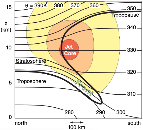
Figure 12.34 Idealized vertical cross-section through the jet stream in N. Hemisphere. Shading indicates west-to-east speeds (into the page): yellow ≥ 50 m s^–1, tan ≥ 75 m s^–1, orange ≥ 100 m s^–1. Thin lines are isentropes (K). Thick line is the tropopause. “Front” indicates the upper-tropospheric front, where stratospheric air is penetrating into the troposphere.

Upper-tropospheric fronts are also called upper-level fronts, and are sometimes associated with folds in the tropopause. A cross-section through an idealized upper-level front is sketched in Fig. 12.34.

In the lower troposphere, the south-to-north temperature gradient creates the jet stream due to the thermal wind relationship (see the General Circulation chapter). A reversal of the meridional temperature gradient above 10 km in this idealized sketch causes wind velocities to decrease above that altitude. Within the stratosphere, the isentropes are spaced closer together, indicating greater static stability.

South of the core of the jet stream, the tropopause is relatively high. To the north, it is lower. Between these two extremes, the tropopause can wrap around the jet core, and fold back under the jet, as sketched in Fig. 12.34. Within this fold the isentropes are tightly packed, indicating an upper-tropospheric front. Sometimes the upper-level front connects with a surface front (Fig. 12.19).

Stratospheric air has unique characteristics that allow it to be traced. Relative to the troposphere, stratospheric air has high ozone content, high radioactivity (due to former nuclear bomb testing), high static stability, low water-vapor mixing ratio, and high isentropic potential vorticity.

The tropopause fold brings air of stratospheric origin down into the troposphere. This causes an injection of ozone and radioactivity into the troposphere. The dry air in the tropopause fold behind the cold front is often clearly visible in water-vapor satellite images of the upper troposphere.

The heavy line in Fig. 12.34 corresponds roughly to the 1.5 PVU (potential vorticity units) isopleth, and is a good indicator of the tropopause. Above this line, PVU values are greater than 1.5, and increase rapidly with height to values of roughly 10 PVU at the top of Fig. 12.34. Below this line, the PVU gradient is weak, with typical values of about 0.5 PVU at mid-latitudes. PVU is negative in the Southern Hemisphere, but of similar magnitude.

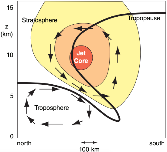
Figure 12.35 Transverse (cross-jet-stream) circulations (arrows) that dynamically form an upper-tropospheric front (i.e., a tropopause fold).

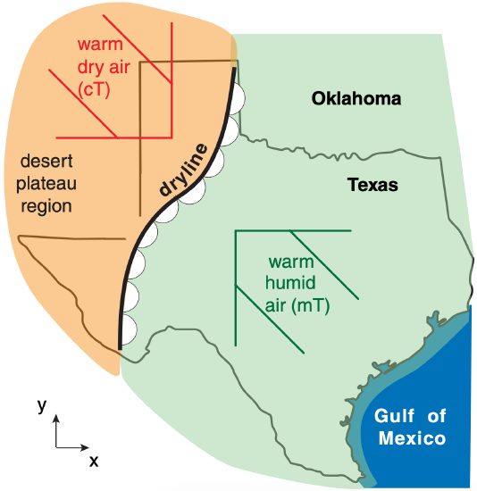
Figure 12.36 Typical location of dryline in the southwestern USA.

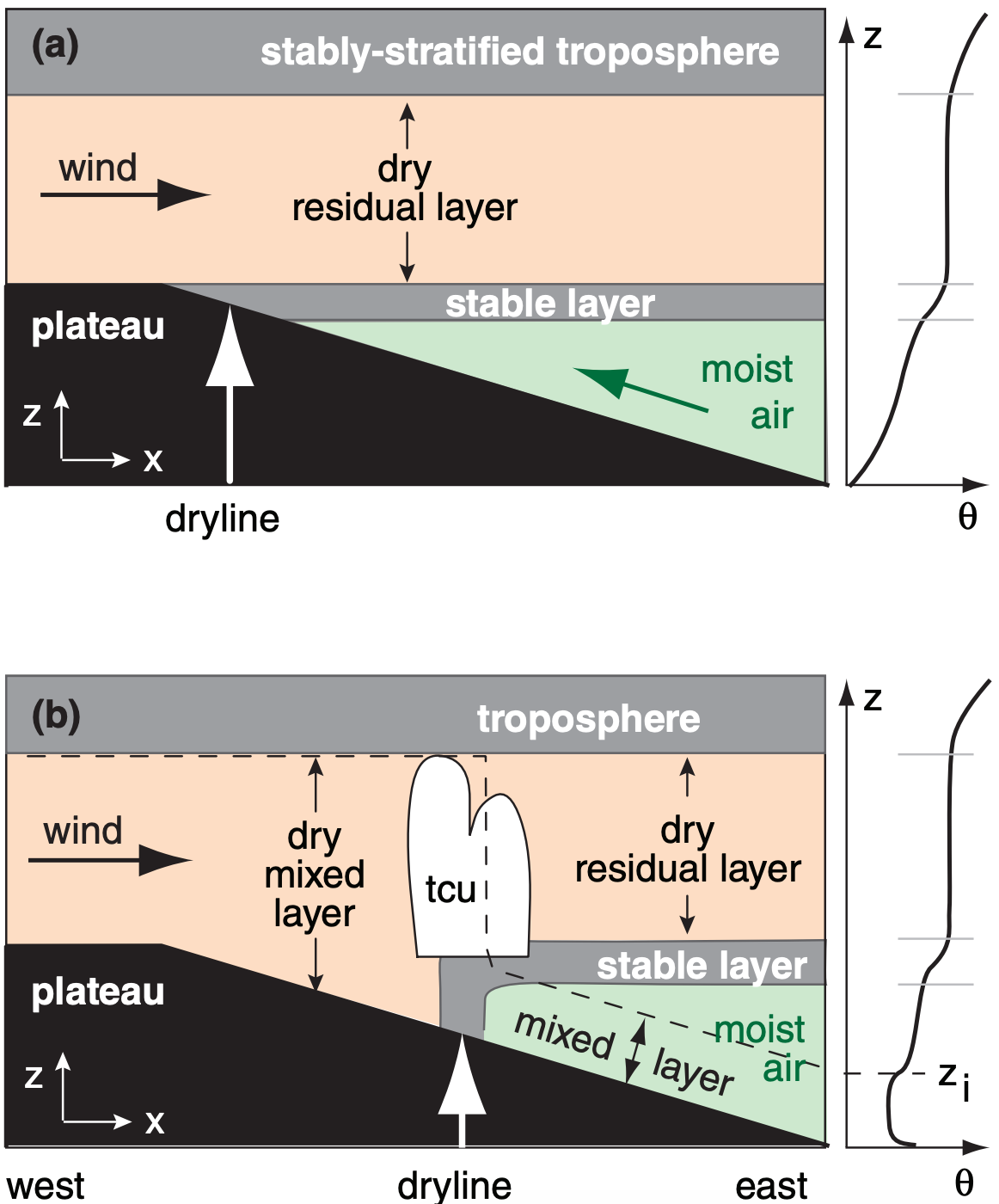
Figure 12.37 Idealized vertical cross section through a dryline (indicated by white arrow). Winds are indicated with black arrows. (a) Early morning. (b) Mid afternoon, with a convective mixed layer of thickness z_i . tcu = towering cumulus clouds. At right of each figure is the potential temperature θ sounding for the east side of the domain.

Sawyer-Eliassen dynamics help create tropopause folds. Picture a tropopause that changes depth north to south, as in Figs. 11.35 or 11.37 of the General Circulation chapter, but does not yet have a fold. If the jet core advects colder air into the region, then the thickness between the 10 and 20 kPa isobaric surfaces (Fig. 11.37b) will decrease as described by the hypsometric equation. This will cause greater slope (i.e., greater height gradient) of the 10 kPa surface near the jet core. This temporarily upsets geostrophic balance, causing an ageostrophic circulation above the jet from south to north.

This transient flow continues to develop into a cross jet-stream direct circulation that forms around the jet as sketched in Fig. 12.35 (similar to Fig. 12.28b). Below the fold is an indirect circulation that also forms due to a complex geostrophic imbalance. Both circulations distort the tropopause to produce the fold, as sketched in Fig. 12.35, and strengthen the upper-level front due to the kinematic tilting term.