38.5: Fossil fuels

Buried carbon does not necessarily stay buried. Our species has found it useful to extract carbon-rich gas, liquid, and solid compounds from the crust and set them on fire. By oxidizing that carbon, we release energy originally bound up in chemical bonds as much as ~350 million years ago. We refer here to and coal, petroleum, and natural gas: the “fossil fuels.” They get this name because all the carbon in each fuel came originally from living things extracting \(\ce{CO2}\) from the atmosphere. Fossil fuels would not exist without life. (Fossils are the remains of ancient life.) Specifically, ancient bog and swamp plants were the precursors for coal, and ancient phytoplankton were the precursors for petroleum and natural gas.

Coal

Figure \(\PageIndex{1}\): Bituminous coal. (Ralph & Cheryl Dawes photo.)

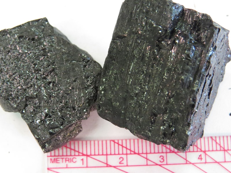
Coal is a solid fossil fuel that forms from compressed plant matter called peat. Frequently coal layers (“seams”) still retain the impressions of leaves, stems, seeds, spores, and other botanical details. Coal comes in several “grades” that reflect varying degrees of compression. The lowest grade is lignite (brown coal), which is just a step up from peat, the original mix of plant bits. If it is more compressed still, it will become bituminous coal. And the highest grade of coal, anthracite, forms only when a coal seam is subject to metamorphism under the influence of mountain-building.

Figure \(\PageIndex{2}\): A peat slide in Shetland, U.K. This cool, wet climate supports the growth of peat, but not trees. Note that the hillside is not a “swamp.” (Callan Bentley photo.)

The plants that are the progenitor of coal live on the land, in wet, aquatic, or swampy settings. It’s traditional to think of coal as coming from swamps, since swamp water is usually stagnant, and thus poorly oxygenated. Carbon-rich plant fragments falling into that water are therefore more likely to avoid oxygenation long enough to be buried. The rate of new carbon being added as plants shed debris outstrips the rate at which oxygen diffuses across the calm surface of the water.

But peat can also form in cool, wet climates such as Ireland or Scotland. There, a layer of vegetation clings to the topography of the land. The damp weather means that sphagnum and heather, the main peat-building vegetation, grow on slopes and hilltops as well as in the valley bottoms, with underlying peat layers averaging a meter or two thick. The entire landscape is essentially blanketed in bog. It grows upward at about 1 cm/year.

Oil

Figure \(\PageIndex{3}\): Distillate of ancient algae, good for powering a civilization. (Callan Bentley GIF.)

Oil has a different origin story. Here, the photosynthesis was conducted by marine or lake algae, phytoplankton floating as single-celled organisms in the uppermost, sunlit portion of the water column. When they died, their bodies rained down to the bottom. This transferred the carbon they contained to the dark depths. Often, the bottoms of lakes or the ocean have far less dissolved oxygen than waters closer to the surface. As a result, carbon entering these anoxic waters tends to be buried before it can oxidize. As with swamp coal, it’s a case of the carbon burial rate exceeding the flow of dissolved oxygen to the same place.

Once buried, the algae have to be warmed up to a critical temperature – about 100\(^{\circ}\)C, the temperature of a freshly made espresso. If it’s too cold, their little dead cells won’t transform into petroleum. If it’s too hot, the mixture will turn into natural gas (described below) and graphite. The temperature has to be just right.

Figure \(\PageIndex{4}\): The Conodont Alteration Index of Anita Harris (then Anita Epstein), et al., 1977. (USGS image.)

Interestingly, one way geologists can make a quick but accurate assessment of the temperature to which potentially-oil-bearing rocks have been warmed is by examining fossils. Specifically, the spiky “elements” of the conodont animal. These are made of hydroxylapatite, a phosphate mineral. The key thing to know about hydroxylapatite is that it changes color when heated, like a piece of toast. Geologist Anita Harris developed a vital tool with the Conodont Alteration Index, a 6-point color scale that uses the various “toastings” of conodonts to see if their host rocks warmed up to the appropriate temperature for oil generation.

Conodonts can then be collected from numerous sites in a region, their color assessed using the Index, and then the presence of each color can be contoured. Here’s an example for the sedimentary strata of the Appalachian Plateaus + the Valley & Ridge provinces:

Figure \(\PageIndex{5}\): Conodont Alteration Index color distribution across the Appalachian Basin. (Modified from a USGS figure.)

Once produced, oil must migrate to a spot where it can collect in amounts where humans will find it economically worthwhile to drill it out and extract it. There are plenty of places where oil naturally seeps out at Earth’s surface, such as the legendary tar pits of Rancho La Brea in Los Angeles, California.

Figure \(\PageIndex{6}\): An anticlinal petroleum trap. (C.Bentley modification of an original diagram by GreenMagenta via Wikimedia.)

But the oil you burn in your automobile found a stable residence underground in some variety of subterranean oil trap. These have various shapes due to various geological circumstances, but one of the easiest to grasp is that of an anticline. If the arch-like shape of an anticline consists of a stack of layers with carbonaceous source rocks at the bottom (such as black shale), impermeable cap rock strata (such as shale) at the top, and a spongey reservoir layer (such as sandstone) in between, that makes for an ideal petroleum trap. Petroleum geologists are charged with finding these traps and directing the company’s engineers to tap into them.

Natural gas

Figure \(\PageIndex{7}\): Outcrop of the Devonian-aged Marcellus Shale in Pennsylvania. Yellow field notebook for scale. (Modified from a Terry Engelder photo.)

Our third and final fossil fuel is neither a solid like coal, nor a liquid like oil. Instead, it’s a mixture of gases, principally methane (\(\ce{CH4}\)). Like oil, its progenitor is phytoplankton. While these algae live, they photosynthesize. When they die, their bodies rain down into anoxic deep waters, imparting a high carbon content to the sediments deposited there. Typically, the resulting rock is a black shale.

Black shales are more common in the geologic record during times of sluggish ocean circulation or widespread stagnation, such as the end-Permian or the mid-Cretaceous. Black shales can also be deposited in lakes; they are not necessarily marine in origin.

Figure \(\PageIndex{8}\): Wells producing natural gas from the Devonian-aged Marcellus Shale. (US Energy Information Administration map.)

The Marcellus Shale of the Appalachians and the Bakken Shale of the Dakotas are both Devonian-aged black shales with lots of natural gas trapped inside them. In the past decade, the advent of horizontal drilling has allowed fossil fuel companies to drill into these shales and intentionally shatter them, allowing the gas to flow out, up the drill hole, where it can be collected, transported, and sold. The shattering process is achieved by (a) injecting fluids under very high pressures, along with (b) sand, which props open the fractured shale once the cracks open up. This process is called hydraulic fracturing, or “fracking.”

Natural gas is also produced in coal seams. This variety is referred to as “coal-bed methane.” Coal miners have been very conscious of coal-bed methane since coal mining began – because it is invisible gaseous reduced carbon, one spark from mining equipment could trigger an explosion. Far too many miners lost their lives to this hazard. They called it (and any other inflammable gas) “firedamp.”