11.2: "The Big Five"

Figure \(\PageIndex{1}\): Marine animal family diversity over the Phanerozoic Eon of geologic time. The “Big Five” mass extinctions are indicated, as well as the Cambrian Explosion and Great Ordovician Biodiversification Event. (Graph by Callan Bentley (2022), after Sepkoski (1984, 2002).)

Traditionally, historical geologists have recognized five major episodes of mass extinction from the fossil record. They show as big spikes on the graph above. Plotted a different way, they show as sharp declines on the diversity through time graph. Chronologically, they are the end-Ordovician extinction, the late Devonian, the end-Permian (which closes the Paleozoic Era), the end-Triassic, and the end-Cretaceous (which closes the Mesozoic Era). Each has its own idiosyncratic circumstances, cast of characters, and potentially unique causes for so much dying. Let us now recap each of them.

Extinction is going on all the time. In a way, it’s arbitrary to select a handful for consideration, both because of the incomplete nature of the fossil record (such as microbial turnover during the Great Oxygenation Event) and background extinctions (such as the spikes you see in the Cambrian above, which seem big because the total known number of fossil organisms was itself low).

End-Ordovician extinction

At the end of the Ordovician period, the only animals on Earth were invertebrates living in the ocean. Certain varieties of mollusks, trilobites, graptolites, eurypterids, brachiopods, conodonts, corals, echinoderms, and other groups all went extinct about 443 Ma. These were all key members of the Paleozoic Fauna. Of the species paleontologists have documented, about 52% of them disappeared at the Ordovician/Silurian boundary, never to return. It is worth emphasizing that — uniquely among the Big Five — the end-Ordovician extinction was entirely limited to marine organisms, since land had yet to be colonized at that time.

The Ordovician/Silurian boundary was defined by Charles Lapworth with the stratotype at Dob’s Linn, Scotland, which is still used as a GSSP today. Below are some of the graptolites Lapworth used as index fossils to distinguish between the two periods in the black shale there:

(Callan Bentley GIGAmacro)

After the mass extinction was over, it took 50 million years for Earth’s oceans to recover their former levels of diversity.

Figure \(\PageIndex{2}\): Faceted and striated clast extracted from Ordovician strata in Arabia. (Modified from Figure 3 of Masri (2017).)

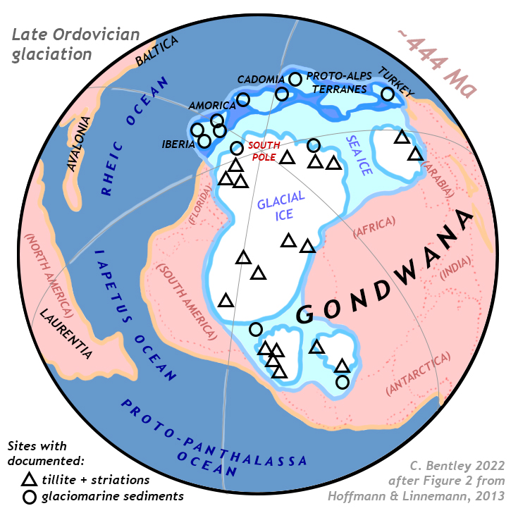
The cause of the late Ordovician extinction is inferred to likely be global cooling. There is evidence of glaciation during the late Ordovician in the southern supercontinent Gondwana: this is known from sedimentological documentation of tillites bearing faceted, striated clasts, and dropstones in what is today South America, Arabia and Africa). There are also vast areas where the glaciers appear to have bulldozed pre-existing unlithified sediments, deforming them as the ice flowed along. Using isotopic evidence, Finnegan et al. (2011) have estimated that global seawater temperatures dropped 5 \(^{\circ}\)C during the latest Ordovician. Five degrees may not sound like much, but because of water’s exceptional heat capacity and the huge volume of Earth’s seawater, it represents a truly enormous amount of heat energy lost from the world ocean. Glass sponges, a deep-water siliceous sponge-like animal, are well-adapted to cold conditions, and they do well in the aftermath of the end-Ordovician extinction.

Figure \(\PageIndex{3}\): Map showing the inferred extent of end-Ordovician glaciation in Gondwana. (Map by Callan Bentley, redrawn after an original by Hoffmann and Linnemann, 2013.)

How could a cooling climate trigger a mass extinction? One key variable is a change in the ocean temperature, with negative impacts for those organisms who are specialized for warmer waters. This is particularly acute in the tropical/equatorial regions of the planet’s ocean. But another key impact is in the change in sea level that accompanies the build up of glacial ice mass. Glaciers are made of water, and that water has to come from somewhere. As we are currently seeing in modern times, melting glaciers add water to the ocean, which raises sea level. The reverse is also true: at the height of the most recent ice age, sea level was ~120 meters lower, and the shoreline was at the edge of the continental shelf. This is bad news for marine invertebrates, most of which live in the shallow marine realm. Dropping sea level by more than 330 feet reduces the amount of habitat they have in which to dwell, and increases competition between individuals.

What caused the cooling climate? It appears to be a coincidence of several events: (1) the position of Gondwana over the south polar region, drifting there due to plate tectonics, and (2) a lowering of greenhouse gas levels through some perturbation to the climate. We can break condition “2” down further into a couple of hypotheses: (2a) enhanced silicate weathering by rainwater carbonic acid due to an episode of mountain-building in ancestral North America, the Taconian Orogeny, and (2b) reduced sunlight influx due to stratospheric dust kicked up by a series of meteorite impacts. These aren’t necessarily mutually exclusive, of course. Let’s briefly examine each.

Figure \(\PageIndex{4}\): The Taconian Orogeny shed off a large amount of clastic sediment, reflecting the weathering and erosion of the late Ordovician-aged Taconian Mountain Range. Much of this sediment was clay, which requires carbonic acid to produce, removing \(\ce{CO2}\) from the atmosphere. (Callan Bentley cartoon.)

The Taconian Orogeny, first phase of the three-part suite of Appalachian Orogenies, was caused by the collision of a volcanic island arc in the Iapetus Ocean with the Iapetan margin of ancestral North America. This raised a big chain of mountains that stretched from Maine to Georgia, and shed a tremendous quantity of clastic sediment, including a lot of mud. Mud is made mainly of clay minerals, which are produced through the hydrolysis of feldspars. Mountain belts put a lot of feldspar into the path of chemical weathering, which gobbles up \(\ce{CO2}\) from the atmosphere.

Figure \(\PageIndex{5}\): The Österplana 065 meteorite is preserved as an inclusion in Ordovician limestone, Sweden. (Modified (enhanced!) by CB from an original by Shmitz, et al. 2016.)

Another possibility has an extraterrestrial component. For a long time, it was observed in limestone quarries in Sweden that there were a lot of meteorites included in those carbonate strata. More widely and generally, sedimentary rocks of that time contained a lot of chromite grains that were attributed to meteors. These meteorites generally share a common composition; they are classified as “L-chondrites,” and are all inferred to come from the breakup of a single chondritic parent body, floating somewhere out in space, at about 468 Ma. There are a lot of them; the profusion of meteorites and chromite grains has been dubbed the Ordovician Meteor Event. The idea is that these meteorites would have kicked up a lot of dust. If that dust reached the stratosphere, where there is no rain or weather, then it could have blocked incoming sunlight. A reduction in the flux of sunlight would have acted to cool the climate, regardless of what greenhouse gases were doing at the time of impact.

So, to summarize: it looks like the first of the Big Five mass extinctions was driven by global cooling.

Late Devonian extinction

Figure \(\PageIndex{6}\): Dunkleosteus, a predatory placoderm from the Devonian. (Public domain.)

After the relatively brief Silurian period (total duration only 20 million years), the planet entered the Devonian period, sometimes dubbed “the age of fishes.” This was a time of great radiation among the fishes, producing the first jawless fishes, sharks, placoderms, the first ray-finned fish, and the lobe-finned fishes, some of whom were almost certainly the ancestors of the humans reading this case study.

Figure \(\PageIndex{7}\): Jawless fish that lived during the Silurian and Devonian periods: tolypelepids (top right), pteraspidids (bottom right), protopteraspidids (bottom left) and the huge psammosteids (top left), which are the only members of the group to survive the late Devonian mass extinction. (CC-BY; Drawing by Phillipe Janvier (1997).)

Toward the end of the Devonian, things started getting rough for organisms on Earth, but unlike the end-Ordovician, end-Permian, end-Triassic, and end-Cretaceous extinctions, this one took a while. It was spread out over more than 20 million years, maybe as many as 25 million. It’s not the called the “end”-Devonian, for that reason. It took a while. It got worse, and then a little better, and then worse again. The two biggest die-offs occurred at 374 Ma and 359 Ma.

Figure \(\PageIndex{8}\): Atrypa reticularis, from Devonian strata in Germany. (CC-BY; Dwergenpaartje photo, via Wikimedia.)

By the end of it, though, 99% of reefs had been destroyed, the diverse fish world had been severely cut back, and many marine groups had been severely pruned back or eliminated altogether. Among reef-builders, the tabulate and rugose corals got slammed. Conservative estimates put the carnage at a 40% loss of taxa. The atrypid brachiopods, for instance, were a diverse tropical group of articulate brachiopods that were extinguished. Moving into their shallow-sea habitat after the extinction were silica-skeleton sponges, which otherwise prefer cooler, deeper water.

One of the first clues that things were going awry in the late Devonian is a profusion of black shales. Black shale is rich in organic carbon.

Figure \(\PageIndex{9}\): Watkins Glen, near Ithaca, New York, is a gorge cut into Devonian black shale of the Genesee Group. (CC-BY; Photograph by Barbara Friedman, via Flickr.)

Carbon loves to react with oxygen, if there’s any oxygen around to react with. If there is, it becomes \(\ce{CO2}\) gas, and diffuses into the atmosphere (and is thus *not* preserved in sedimentary rock). But if muddy sediment is deposited under low-oxygen or anoxic (no oxygen) conditions, any organic carbon will be interred in the sedimentary record, giving its host rock a dark gray or black color.

So why was so much of the ocean anoxic in the late Devonian? The answer may surprise you: trees.

Figure \(\PageIndex{10}\): The roots of this tree are demonstrating the destructive power of root wedging. Though this picture is an anthropogenic “rock” (asphalt), it works on natural rock as well. (Public domain image.)

Yes, you read that right: trees. During the Silurian, the first plants [LINK TO PLANTS CASE STUDY HERE] had colonized wet areas of the shoreline of freshwater areas. Mosses and liverworts can’t do much in terms of churning into their sedimentary substrate, but trees can. During the Devonian, Earth’s land surfaces saw the growth of the first forests. The trees in these forests had roots, and those roots probed down into the ground, helping break up rocks below, and thereby releasing their nutrients at an accelerated rate. Organic acids produced by the trees probably helped accelerated chemical weathering, too.

Figure \(\PageIndex{11}\): Eutrophication of the Potomac River adjacent to a wastewater input. (CC-BY; Photo by Alexandr Trubetskoy.)

While the trees doubtless consumed some of these liberated nutrients themselves, others were washed away by streams and rivers, ending up in the oceans. Today, agricultural use of phosphorus and nitrogen fertilizers produces a similar kind of nutrient-rich runoff. When it reaches the ocean, this “vitamin soup” jacks up the rate of reproduction of algae; a process called eutrophication. At this point, it all sounds well and good. The issue that makes it deadly enough to cause a mass extinction, though, is that when those supercharged populations of algae die, they die in great numbers. The rotting those billions of dead algae cells consumes all the available oxygen in the water, creating “dead zones” which lack dissolved oxygen. Any fish swimming into such a dead zone must turn around immediately, or asphyxiate. Sadly, this happens regularly today in places like the Gulf of Mexico, where the Mississippi River efficiently delivers nitrogen and phosphorus washed off farm fields in the central United States. Human sewage is another rich source of nutrients; when it enters freshwater lakes or rivers, it can drive this same harmful “boom and bust” cycle that depletes the water of oxygen.

Once the supply of oxygen was exhausted, remaining unrotted dead algae rained down on the seafloor in profusion. Hence: a lot of black (organic-rich) shale. You may have heard of fracking, the process by which humans use high-pressure fluids to shatter organic-rich rocks deep underground, allowing natural gas to flow out. The targets for those fracking operations are mostly Devonian black shales. The Bakken Shale in North Dakota, and the Marcellus Shale in western Pennsylvania are today enticing targets for natural gas exploration because of events that occurred during the late Devonian mass extinction.

Figure \(\PageIndex{12}\): Carbon and oxygen fluxes between plants, the atmosphere, and the geosphere. Carbon burial during the late Devonian drew down atmospheric \(\ce{CO2}\) levels. (Callan Bentley cartoon.)

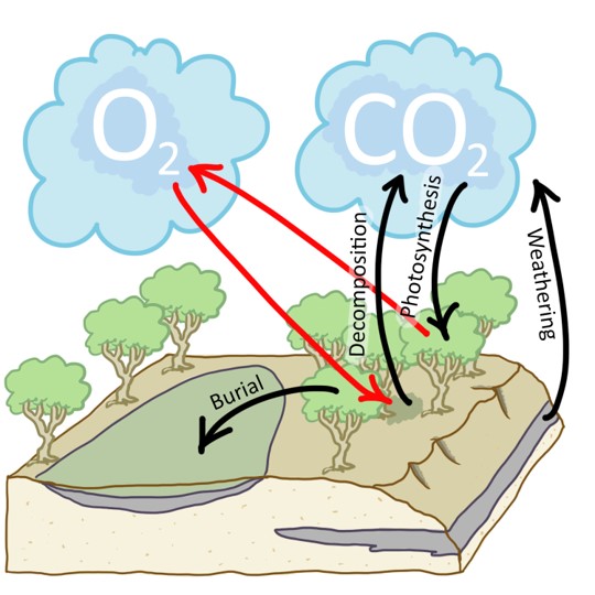
So that is part of the story, but producing thousands of cubic miles of black shale has implications for the planet’s climate, too. Removal of all that organic carbon from the biosphere means that the atmosphere will be relatively depleted in \(\ce{CO2}\), which is of course a greenhouse gas, helping warm the climate. When \(\ce{CO2}\) levels are drawn down, there’s less heat retained by the planet, and global cooling can result.

As with the end-Ordovician extinction, there is evidence for a new build-up of glacial ice during the late Devonian. In the Appalachian basin of Maryland, Pennsylvania, and West Virginia, distinctive glaciogenic sedimentary layers can be observed from the late Devonian. Given that paleomagnetic reconstructions put this part of ancestral North America about 30\(^{\circ}\) south of the equator at the time, this implies fairly cold conditions indeed!

As with Snowball Earth, the end-Ordovician glaciation, or the Pleistocene “ice age,” the evidence of glaciation can be seen in faceted, striated clasts, tillites, and dropstones.

Figure \(\PageIndex{13}\): Outsized granite cobble in black shale of the latest Devonian Rockwell Formation, Grant County, West Virginia. (Callan Bentley photo.)

Figure \(\PageIndex{14}\): The “Robinson boulder,” (Logan Branch, Morehead, Kentucky) is a faceted, granite dropstone estimated to weigh 3 tons. It is embedded in the anoxic Cleveland Member of the Ohio Shale (late Devonian). Note upturned layers or “mud drape” along edges of the boulder. Hammer for scale. (From Ettensohn, et al. (2020); reproduced with permission.)

Just to bring the discussion of the late Devonian mass extinction full circle, consider anew the black shales laid down on the seafloor, robbing the Devonian atmosphere of its warming \(\ce{CO2}\). As we extract and burn natural gas from these shales today so that we may produce energy, we *finally* oxidize all that fossil carbon, which had remained sequestered underground for more than 300 million years and would have continued to do so if industrialized humans hadn’t shown up. The \(\ce{CO2}\)-induced warmth that would have saved the Devonian biota from an ice age is now being unleashed on the Holocene (and maybe inducing the Anthropocene...).

End-Permian extinction

Figure \(\PageIndex{15}\): Fusulinid foram fossil from Permian limestones in west Texas. (Callan Bentley photo.)

The end-Permian mass extinction was the most extreme of any in Earth history. It’s sometimes dubbed “The Great Dying,” with 62% of marine genera going extinct, as well as severe impacts among terrestrial biota. Perhaps only 17% of species on Earth survived it. It’s the sharp cliff at the end of the “Paleozoic Plateau.” It’s the closest our biosphere has ever come to being deleted. Writer Peter Brannen astutely called it “the worst thing that ever happened.”

By the end of the Paleozoic, life had rebounded from the late Devonian extinction. In the sea, crinoids and their cousins the blastoids were having a heyday. Tabulate and rugose corals had made great progress in building up reefs in the late Paleozoic ocean, reefs that almost certainly served as shelter and nurseries for many other species, as modern scleractinian coral reefs nurture fish, shrimp, crabs, etc. Giant single-celled fusilinid foraminiferids were rolling around the seafloor like fat grains of rice.

Figure \(\PageIndex{16}\): Dimetrodon reconstruction. The posture is controversial, but here shown upright, based on possible Dimetrodon trackways. (Max Bellomio imagery, via Wikimedia.)

On land, the Glossopteris seed fern reigned supreme, at least over the southern supercontinent Gondwana. In its shade, the waterproof amphibian descendants called reptiles had diversified and spread into a great number of ecological roles. Dominant among them were the synapsids, those that used to be dubbed “mammal-like reptiles.” In some cases, these animals could grow to large sizes. You would not have wanted to meet Dimetrodon in a dark alley. The sail-like “fin” rising from its back is its most eye-catching feature, but its mouth was full of sharp teeth.

Also worth noting are the cynodonts, which are probably the direct ancestors of the mammal lineage. Cynodonts were not as large as the therapsids, though, and many of them were hungry. With massive heads bearing powerful jaws and saber-like teeth, Gorgonops and its kin were fearsome beasts. The therapsids had several advantages over their less derived pelycosaur relatives. They had a fully-upright stance, with their limbs always beneath the body. There is also potential evidence that they were endothermic (also called ‘warm-blooded’) and had at least some hair. Many species show ‘whisker pits’ in the skull, which is good bony evidence of hairs that were once anchored in these pits.

Figure \(\PageIndex{17}\): Gorgonops, a large Permian predatory therapsid. (Reconstruction by Dmitry Bogdanov via Wikimedia.)

Another group of reptiles had a relatively subdued presence during the Carboniferous and Permian: the sauropsids. These animals included the ancestors of modern lizards, snakes, crocodiles, and birds, as well as the dinosaurs who would dominate the Mesozoic.

Figure \(\PageIndex{18}\): Lystrosaurus murrayi, about the size of a small dog. (CC-BY; Sketch by Dmitry Bogdanov, via Wikimedia.)

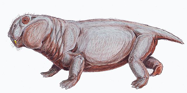
Gorgonops and Dimetrodon went extinct at the end of the Permian, along with 2/3 of therapsids. Some cynodonts survived, and these diversified during the Mesozoic that followed, some of them ultimately leading to you and me. One that practically overran the world in the early Triassic was Lystrosaurus, whose populations rose unchecked after the the demise of all its predators. But in the Mesozoic, it was the sauropsids that diversified most successfully, and led to dinosaurs, plesiosaurs, ichthyosaurs, pterosaurs, and mosasaurs. They were the big winners from the end-Permian extinction. But there were so many losers...

Figure \(\PageIndex{19}\): El Capitan and the Guadalupe Mountains of west Texas, a Permian reef complex and the namesake of the Guadalupian epoch of the Permian period. (Public domain; NPS photo.)

There were two pulses to the end-Permian extinction. Because they were separated by ~8 million years, it has become commonplace in recent years to hear them discussed independently: the Capitanian (or ‘end-Guadalupian’) at 260 Ma and the true end-Permian event at 252 Ma. Both appear to have the same general cause: global warming.

The careful study of variations in oxygen isotopes in strata spanning the Permian-Triassic boundary shows an lightening of the oxygen content of the oceans. This correlates with a big boost in heat energy, making \(\ce{^{18}O}\)-based water molecules as likely to evaporate as \(\ce{^{16}O}\)-based water molecules. Using the ratio of \(\ce{^{16}O}\) to \(\ce{^{18}O}\), it has been calculated that the global ocean warmed by about 6 \(^{\circ}\)C. As with the discussion of ‘cooling by 5 \(^{\circ}\)C’ in the end-Ordovician extinction above, please realize that it takes a truly enormous amount of energy to shift ocean temperatures by six whole degrees Celsius. That extra energy would have been radiated to space, had it not been trapped by extra \(\ce{CO2}\) in the late Permian atmosphere.

Now let’s consider where that extra \(\ce{CO2}\) came from, and then examine the havoc it caused in the ocean.

There were two major large igneous provinces that erupted during the late Permian. The first was in China: the Emeishan Traps, where “Traps” derives from the Swedish word trappa, meaning “stairsteps.” This refers to the step-like landscape where the many layers of a vast flood basalt province get etched out. (The Deccan Traps in India have a similar morphology, as do the lava layers of the Columbia Plateau in eastern Washington state.) The Emeishan basalts erupted from 265 to 259 Ma.

Figure \(\PageIndex{20}\): Putorana Plateau, Russia, part of the Siberian Traps flood basalt province. (CC-BY; Photo by Александр Лещёнок, via Wikimedia.)

The second, much larger, was in Siberia. Today we call it the Siberian Traps. The Siberian Traps represents one of the biggest eruptive episodes in Earth history. Presumably the result of a mantle plume slamming into the bottom of the north Asian continent, the volcanic rocks of the Siberian Traps have been shown to span the Permian-Triassic boundary, including the mass extinction at 252 Ma.

Figure \(\PageIndex{21}\): Roughly what Siberia looked like 252 million years ago. (From a video by the USGS.)

Size estimates of the Siberian Traps boggle the mind: A volume of more than 1.5 million cubic kilometers of lava was erupted, smothering roughly 2 million square kilometers of northern Siberia. That is enough basaltic lava to bury the entire contiguous United States to a depth of half a mile. It’s enough basalt to make three towers, each with a footprint of 1 square kilometer, that reach to the Moon.

So much lava being erupted carries with it a commensurate amount of volcanic gas. Most of that gas is water vapor, which is rapidly removed from the atmosphere via precipitation. But the second most common volcanic gas is \(\ce{CO2}\), and you know what that does.

Not only that, but one of the layers that the Siberian Traps basalt passed through on its way from the mantle to the surface was a vast Carboniferous-aged coal field (the world’s largest) in the Tunguska Basin, which caught fire and burned, adding even more \(\ce{CO2}\) to the total that was released! Estimates are that the level of \(\ce{CO2}\) in the atmosphere reached to at least 3000 ppm, and maybe as high as 30,000 ppm. Average estimates for the end-Permian are ~8000 ppm. (For reference, in 2022, the world was at about 420 ppm, up from ~280 ppm in pre-Industrial times.) So the end of the Permian had twenty times as much \(\bf{\ce{CO2}}\) in its atmosphere as we do today, an insane level that would have warmed the planet to an astonishing degree.

Figure \(\PageIndex{22}\): Outcrops in Inuyama, Japan, show a Triassic sequence of sedimentary strata that record changes in deep ocean oxygen levels after the end-Permian mass extinction event. The strata have been tectonically rotated due to accretion with the Japanese mainland. (Photo by Yukio Isozaki; reproduced with permission.)

A warm climate doesn’t necessarily spell the end of the world, but in this case, the oceans played a key role. In the modern world, with cold polar regions and warm tropics, our ocean vigorously circulates in a vast, floppy loop. The energy that drives this flow of water comes from the difference in temperature (and thus density) of the water. When warm water grows cold, it gets more dense, and it sinks. Sinking water pulls other water after it, and a flow is induced. But in the Permian, as the polar oceans warmed up to roughly the same temperatures as the tropics, this flow was reduced, and — apparently — stymied completely. In short, the oceans became stagnant.

As with the late Devonian, this produced anoxia in the oceans, which is recorded as usual by jet black sedimentary deposits. The anoxia was at first most pronounced in the deep ocean, but it appears to have eventually invaded the coastal shallows. This is where most marine life makes its home, and that was of course quite disastrous.

Worse, though, is what happened when the Sun’s rays hit the anoxic shallow water. This is the rare combination of factors that promotes the growth of sulfur-reducing bacteria, which release hydrogen sulfide gas (\(\ce{H2S}\)) as a waste product. You know \(\ce{H2S}\): it’s the stink of rotten eggs — or the nauseating stench of really gross farts. In low levels, it’s revolting and annoying, but in high levels, it’s deadly. The appearance in seafloor sediments of little raspberry-shaped clusters of pyrite (\(\ce{FeS2}\)) suggest that the ocean at the end of the Permian was quite rich in sulfur. The inference is that these distinctive purple bacteria must have bloomed in profusion without any of their usual microbial competitors.

Figure \(\PageIndex{23}\): Purple sulfur bacteria from a modern euxinic lake in British Columbia. (J. Glass photo; permission requested.)

Thus the oceans were not only anoxic, but also probably also euxinic — the word that describes being thoroughly infused with \(\ce{H2S}\). In 2005, Lee Kump and colleagues suggested something bold – that the oceans were so euxinic during the end-Permian that \(\ce{H2S}\) began to exsolve out of the sea and into the air, where it acted like an agent of chemical warfare, gassing terrestrial animals to death.

Another potential “kill mechanism” that applies to terrestrial species has its roots in a layer of rock salt that the Siberian Traps eruption also pierced, exploded, and scattered as it erupted. The chemicals that were released are thought to be the sort that destroy ozone (\(\ce{O3}\)), which humans have done using the famous chlorofluorocarbons (CFCs) that were banned by the Montreal Protocol. If the stratosphere’s ozone layer was severely damaged at the end of the Permian, that would have increased the flux of ultraviolet light (particularly UV-B) to the surface of the planet. This deadly radiation would have potentially driven up rates of mutations and cancers for any organism that was exposed to it (i.e., only those who lived on land).

Figure \(\PageIndex{24}\): A layer of limestone made of nothing but shells of the clam Claraia. (Modified from a photo by Toedi3614, via Wikimedia.)

In the aftermath, the world lay obliterated, an apocalyptical denuding of the biosphere that probably reeked of rotten eggs. On land, the formerly terrifying forms of Dimetrodon and Gorgonops lay still; corpses rotting away in the foul air. The forests of sphenopsids and lycopsids were done forever. From the rotting foliage, a few therapsids nosed out and sniffed the air. In the sea, there were no more blastoids, no more fusulinid forams, no more trilobites or rugose corals. No more eurypterids; no more goniatitic ammonoids. Brachiopods were greatly reduced in number and diversity (a 96% decline). They would be replaced by the bivalves in the years to come. Still depleted in oxygen and utterly emptied out, the early Triassic seas were overtaken by one genus of clam that was adapted to low-oxygen conditions. Claraia spread far and wide, unimpeded by any competition. It’s so omnipresent and numerous that as a monoculture, it makes an excellent index fossil for the first part of the Triassic period: a bizarro “Clamworld.”

This was the one big reset of Earth’s biosphere –phyla that had dominated the oceans for 200 million years were gone, and oceans would never look the same. The survivors went on to diversify into the Modern Fauna; mollusks would now reign supreme, scleractinian corals would build reefs, and echinoids, sea stars and sea cucumbers would now represent the echinoderms (replacing crinoids and blastoids).

End-Triassic extinction

Figure \(\PageIndex{25}\): The Palisades cliff above the Hudson River in New Jersey is the surface expression of a vast near-surface mafic sill. This massive slug of basalt was intruded into the Newark Basin during the breakup of Pangaea. (CC-BY; Photo by Anita Gould, via Flickr.)

Therapsids flourished in the Triassic, now that their synapsid competitors had been suffocated. These crocodilian relatives were attended by the first dinosaurs, but dinosaurs were the sideshow rather than the main act. Only after the end-Triassic extinction could the dinosaurs surge forward and dominate the Mesozoic land surface. But first, their crocodilian overlords must be cleared away.

In the sea, about half of the Triassic genera didn’t make it into the Jurassic. Almost every kind of ammonoid and bivalve was decimated. Ammonoids had evolved a ceratitic morphology, which is an index fossil for the Triassic. Also in the seas were a menagerie of marine reptiles, many of whom were snuffed out by the end-Triassic extinction event. Walrus-like reptiles called placodonts and the seal-like nothosaurs totally perished, while some of their ichthyosaur and plesiosaur cousins eked a way through, and would re-diversify in the Jurassic and Cretaceous.

Figure \(\PageIndex{26}\): Conodonts were eel-like jawless fish that left behind copious prickly “elements” as index fossils. (Both CC-BY; Photo illustration by C. Bentley (2022), using the background illustration by Nobu Tamura and element photo by Wikipek, both via Wikimedia.)

One small animal of note, the conodonts (a kind of thin, eel-like jawless fish) had been a fixture of Earth’s oceans from the Cambrian onward. They were practically as common in the oceans as water molecules, and left their jaws and gill support structures behind as an uniquely valuable index fossil. But the end-Triassic got them, too. Their long run on Earth came to an abrupt end at 202 Ma.

Now that you know who died and who survived, let’s examine the “why?”

Like the end-Permian crisis that preceded the Triassic, the mass extinction that brought it to an end appears to be a case of (1) “large volcanic province erupts,” (2) “\(\ce{CO2}\) levels spike,” and (3) “global warming ensues.” In this case, a hot spot is not to blame.

Figure \(\PageIndex{27}\): Location of mafic igneous rocks of CAMP in four continents, positioned at the time of Pangaea’s breakup. (Williamborg image, after Blackburn (2013), via Wikimedia.)

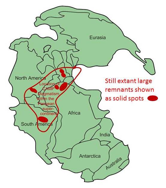
Instead, it was the titanic breakup of the most gargantuan supercontinent ever. As rifting split Pangaea and opened the spindly Atlantic Ocean down its center, the underlying crust was thinned dramatically. In what is today eastern North America, a series of rift basins — the Newark Supergroup basins — opened up along normal-faulted hinges, dropping down like trap doors. These basins did an excellent job catching immature sediment from the surrounding highlands, but they also released the pressure on the hot mantle beneath, which partially melted and made its way upward along the fault system. What issued forth was an enormous amount of basaltic magma. And it wasn’t only in North America; huge quantities of basalt and gabbro were produced in adjacent regions of northeastern South America, northwestern Africa, and southwestern Europe. Though its various major volcanic centers have now been separated by seafloor spreading of the Atlantic Ocean, they were once adjacent. Today we call it all the Central Atlantic Magmatic Province (CAMP).

Ultimately, CAMP may have erupted even more basalt than the Siberian Traps, but a good amount of it has since weathered away. Its total volume is estimated at something between 2 and 3 million cubic kilometers of mafic igneous rock. CAMP rocks cover 11 million square kilometers. The eruptions came in four major pulses over the span of about 600,000 years. That’s a lot of magma making it to the surface (and degassing \(\ce{CO2}\)) in a relatively short amount of time.

Figure \(\PageIndex{28}\): Colorized scanning electron micrograph of a single stoma on the underside of a tomato leaf. Here, the guard cells are relaxed, and the stoma is closed. (Modified from a public domain image via Wikimedia.)

An interesting study about the Triassic extinction uses plant fossils [LINK TO FOSSIL PLANT CASE STUDY] as a proxy for examining \(\ce{CO2}\) levels at the time. On the underside of plant leaves are little holes that allow gas exchange with the atmosphere. These holes, called stomata (singular: stoma), are like little doors that let \(\ce{CO2}\) in to enable photosynthesis and waste \(\ce{O2}\) out after glucose has been made. In modern plants, the number of stomata inversely correlates with atmospheric \(\ce{CO2}\) levels. The higher the \(\ce{CO2}\) level, the fewer stomata are needed to get what the plant needs. Under conditions of lower \(\ce{CO2}\), plants require more stomata to let in sufficient air to extract the same absolute amount of \(\ce{CO2}\). So simply by collecting fossil leaves and counting their stomata with a microscope, we can arrive at a sense of how \(\ce{CO2}\) levels varied across the Triassic/Jurassic transition. Jennifer McElwain and colleagues (1999) analyzed fossil leaves from end-Triassic strata in Greenland and Sweden. They found that the stomata density decreased dramatically at the end-Triassic, commensurate with an atmospheric \(\bf{\ce{CO2}}\) level that was seven or eight times as high as we have today. That means a 3-4 \(^{\circ}\)C jump in temperature, above and beyond temperatures that were already ~3 \(^{\circ}\)C warmer than today’s. [If you’re interested in this technique, the Smithsonian has a citizen science project for counting stomata that you can help out with.]

With the planet’s biota reset once again, it was finally time for the dinosaurs to have their day.

End-Cretaceous extinction

Figure \(\PageIndex{29}\): “Sue,” the most complete Tyrannosaurus rex fossil, on display at the Field Museum, Chicago.

Dinosaurs came in two major groups, the saurischians and the ornithischians. With the crocodile-like Triassic therapsids now mostly dead, the dinosaurs diversified and persisted for tens of millions of years. They dominated terrestrial ecosystems in a pervasive and enduring fashion. Other reptiles colonized the air (pterosaurs, and eventually birds too) and the sea (plesiosaurs, ichthyosaurs, huge turtles like Archelon, and eventually mosasaurs too). Giant reptiles were everywhere during the Jurassic and Cretaceous. The world was their oyster.

Figure \(\PageIndex{30}\): Display in the Natural History Museum of London, showing ammonoids as the ideal index fossils. (Callan Bentley photo.)

Speaking of oysters, the sea had plenty of those during the middle and late Mesozoic. Some of them encrusted the shells of clams called inoceramids that had shells a meter in diameter. Another bizarre bivalve group was the rudists, which resembled Sesame Street’s Oscar the Grouch in their trashcan-like morphology. Swimming among them were spiral-shelled cephalopods: the ammonitic ammonoids, which bore distinctly fractal-looking suture patterns between segments of their shells. They make for superb index fossils for the Jurassic and Cretaceous. But along with the dinosaurs and other giant reptiles, their time on Earth came to an end on one very bad day.

Before we get to that day, there are several items that need mentioning. First off, the Cretaceous was hot in general, all around the world. There is no evidence of glacial ice anywhere on the planet during this “hothouse” climate. This, combined with a vigorous rate of seafloor spreading, pushed oceans up onto the continents. In North America, this allowed the Western Interior Seaway to develop as the Sevier Orogeny produced an adjacent foreland basin.

Figure \(\PageIndex{31}\): India’s Deccan Traps are made of many layers of flood basalts. (CC-BY; Photograph by Nichap, via Wikimedia.)

Then things started going wrong. The first, you’ll be shocked to hear, was the eruption of another large igneous province. This one was in western India: the Deccan Traps. As with the Emeishan Traps and the Siberian Traps discussed above, this is a landscape of step-like mesas and plateaus, as a thick stack of basalt flows has been dissected by more recent streams. Like them, it is astoundingly large: 1 million cubic kilometers of basalt, slathering half a million square kilometers of western India (it may have originally been much higher in volume and area, but as with CAMP, it looks like much has been eaten away by subsequent erosion). The eruptions were relatively rapid – from beginning to end, it may have lasted only 30,000 years. At the time of its eruption, India was its own small continent, surrounded by the Indian Ocean — i.e., this was prior to its collision with southern Eurasia. It is inferred that the eruptions were triggered by the island continent’s drift over the Réunion hotspot, a long-lived welt in the Earth’s mantle that is still producing lava today, at namesake Réunion Island itself.

Figure \(\PageIndex{32}\): The Cretaceous-Paleogene boundary at Bottaccione Gorge, near Gubbio, central Apennines of Italy. Pencil for scale. (Callan Bentley photo.)

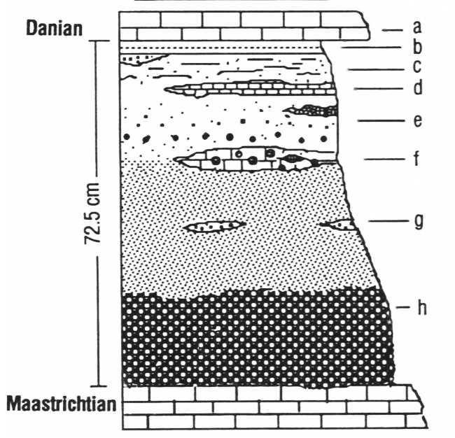
Up until 1980, that alone would have been viewed as entirely sufficient to explain the end-Cretaceous (a.k.a. “K/T” or “K/Pg”) extinction. But in 1980, a son/father team published a paradigm-shifting paper in the journal Science that dredged up the specter of catastrophism anew. Walter Alvarez and his father Luis Alvarez, with others, published a bombshell of a paper that laid out the case for an extraterrestrial impact as the cause of the end-Cretaceous extinction. The younger Alvarez was working as a geologist in the central range of mountains that run down the spine of Italy, the Apennines. He studied the stratigraphy of the limestones and shales there, and one day got to wondering about the nature of the boundary between the Cretaceous and the Tertiary*. He noticed that it really came down to a single layer of clay between two ~4 cm thick limestone strata. He had a really great outcrop in Bottaccione Gorge, a canyon near the town of Gubbio. Below this horizon, Alvarez saw distinctive Cretaceous radiolarian fossils. Above it, none.

* When Alvarez did this work, “Tertiary” was still used as a period by the International Commission on Stratigraphy. Only more recently (2003) did “Paleogene” replace it.

Figure \(\PageIndex{33}\): The iridium anomaly in Italian limestone/shale strata, presented by the Alvarez, et al. (1980) paper. (Graph redrawn by C. Bentley (2022))

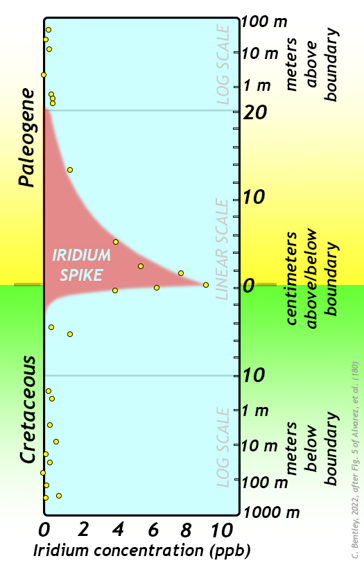
It occurred to him to wonder how much time was packed into that clay layer. Was it 10,000 years, or 100,000, or something else? His father, a Nobel-prize-winning physicist, suggested examining the clay layer from the perspective of the small but (presumed-) constant flux of micrometeorites to Earth. Luis Alvarez advised his son to look for something distinct to outer space sources, that would have built up gradually, and thus could be used to calibrate how much time had elapsed while the clay was deposited. The elder Alvarez suggested the element iridium, which (he hypothesized) should have a more or less constant flux to Earth’s surface.

But the amount of iridium they actually measured were out of this world. Literally.

There was so much iridium packed into that clay layer that the Alvarez team found another hypothesis more likely: this had to be fallout from a single giant meteorite impact somewhere else in the world.

Though many geologists initially were skeptical of this “catastrophe” of a hypothesis, they soon got busy testing it, by checking the Cretaceous/Paleogene (K/Pg) boundary elsewhere in the world, to see if other locations also shared this iridium anomaly. Sure enough: they showed the iridium anomaly, too! In addition, they started documenting additional evidence of an impact: (1) spherules and (2) shocked quartz.

Figure \(\PageIndex{34}\): Grain of shocked quartz viewed under cross-polarized light with a petrographic microscope. Note the planar deformation features. (Public domain; Photograph by Glen A. Izett, USGS.)

Spherules are little glass droplets that form when rock, melted instantaneously by the tremendous heat of the impact, is flung into the air as billions of tiny droplets. These cool and solidify before they rain out onto the landscape: little glass beads that speak of unimaginable violence. Shocked quartz is a little bit different: it starts off as a solid crystal of the common mineral quartz, but then it deforms as the powerful shock wave of the impact passes through it, wrecking its previously precise crystal lattice but not destroying the integrity of the grain by melting or disintegrating it. These distinctive features were first identified in the aftermath of nuclear bomb testing, and were decisively associated with extraterrestrial impacts by the legendary Gene Shoemaker, the “grandfather of impact geology.”

The K/Pg boundary layer thickened toward the Americas, and toward the Gulf of Mexico even more. In their search for oil and gas deposits, the Mexican state petroleum company, Pemex, had mapped a vast circular structure that was mostly under the Gulf of Mexico, but also had about a third of its area lapping over onto the thumb-like Yucatán Peninsula. At first, it was inferred to be a big, extinct volcano, but in 1981, geophysicists Glen Penfield and Antonio Camargo suggested it was an impact crater instead, and indeed that it was the one responsible for the end-Cretaceous extinction. One reporter, Carlos Byars, wrote up the announcement for the Houston Chronicle. Somehow, almost no one noticed.

Luckily, a decade later, Byars was covering a geology conference where the crater’s location was still an enigma. In an astonishing moment, the journalist Byars let the scientists in on what to him must have seemed like “old news” — and now the geological community had found its ground zero, its Big Kahuna.

Figure \(\PageIndex{35}\): The position of the Chicxulub impact structure in the southern Gulf of Mexico and northern Yucatan Peninsula. (C. Bentley annotation of a NASA image.)

The crater was centered on a small port town called Chicxulub. Thus, the structure has come to be known by that name. The structure is about 180 kilometers (110 miles) in diameter and 20 kilometers (12 miles) deep, but it is now mostly hidden from view underneath the subsequent 65 million years worth of sedimentation – limestone, mostly. These overlying limestones have slumped downward a bit over the course of the Cenozoic, allowing a distinctive ring-shaped scarp to develop in the overlying limestone of the Yucatán. All along this ring are water-filled sinkholes, called cenotes. The entire arc of cenotes is a candidate World Heritage Site, not only for its relevance to the end-Cretaceous extinction, but also because the great pre-Columbian civilization of the Mayans utilized these cenotes for access to water.

Impact experts can model the size of the impacting object (a meteorite or a comet, or more agnostically named, a bolide) by the size of the crater it leaves behind. In this case, the impactor would have been about ten kilometers across, roughly the diameter of San Francisco, or Mount Everest. The energy released would have been something on the order of 100 million megatons of TNT. If you’ve seen footage of the Chelyabinsk meteorite’s detonation in 2013 over Russia, you’ve seen what half a megaton looks like. Just multiply that by 200,000,000.

Figure \(\PageIndex{36}\): Part of Figure 1 of Maurrasse & Sen (1991), documenting key stratigraphic features of the K/Pg boundary at Beloc, Haiti. From bottom to top, the strata above the last Cretaceous limestone [Maastrichtian] include (h) coarse, brown, spherule-rich ejecta layer, now converted mostly to smectite clay, (g) fine spherules in sandy marl, (f) coarse-spherule-bearing marl lens, (e) graded sandy marl with small lens of micrite, (d) white chalk lens, (c) laminated sandy marl with small lenses of coarse spherules, (b) fine clay with greatest iridium concentration, (a) earliest Paleogene limestone [Danian].

The “discovery” of the Chicxulub stimulated geological interest immensely – the key elements of the story were now in place. Jan Smit added another: tsunami deposits at the K/Pg boundary at sites in Mexico and Texas. Floretin Maurrasse also documented a substantial tsunami deposit on the island of Haiti.

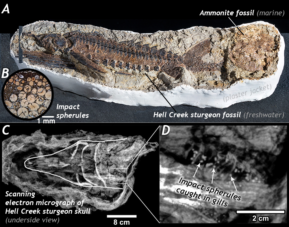
Recently, Robert DePalma and colleagues (including Walter Alvarez and Jan Smit) published a new site they call “Tanis” in North Dakota. It exposes strata of the Hell Creek Formation. Though the Hell Creek is a widespread regional geological unit, Tanis holds an incredible concentration of fossils that appear to have been deposited within hours of the impact. There are many superlative features of Tanis, but one of the most evocative is the presence of meteorite impact evidence inside the organisms fossilized. Specifically, fish breathe with gills, and those gills strain oxygen from the water. At Tanis, about half of the fish fossils have impact spherules caught in their gills, suggesting they were alive and breathing as impact debris was raining down upon their waterway. This astounding details suggests an amazing level of precision for the date of the Tanis deposits – they literally show the very last day of the Cretaceous period.

Figure \(\PageIndex{37}\): Photo illustration showing key details from the Tanis site. (A) shows a fossil sturgeon from the site adjacent to an ammonite; a freshwater species and a marine species deposited at the same moment, in the same stratum (modified from a NASA photo), (B) impact spherules from Tanis, (C) a scanning electron micrograph of the underside of a sturgeon skull, with (D) showing a zoomed-in look at the gills of this poor fish, clogged with impact spherules. (Images B, C, and D are from Figures 4 and 6 of DePalma, et al. (2019).)

So there is now substantial evidence for a major extraterrestrial impact at the very, very end of the Cretaceous. But how did that kill half of life on Earth? Various kill mechanisms have been proposed, including from the radiative heat of the impact, blunt force trauma from its shockwave, subsequent forest fires, violent tsunamis, ocean acidification, and finally a prolonged “nuclear winter” from small particles suspended in the stratosphere. Upending the food chain, some or all of these traumas destabilized the biosphere and ended the Mesozoic Era. What followed was the Age of Mammals, the Cenozoic — the time that would ultimately lead to us.

It’s worth noting that dinosaurs aren’t all gone... birds are with us today, and like mammals and plants (particularly angiosperms), the birds have undergone adaptive radiations to lead to the familiar ecosystems we see across the modern Earth.