13.3: Seasonal Cycles

Substantial seasonal variations in primary productivity occur in middle and high latitudes, but not in the tropics and subtropics (Figs. 12-13, 13-9). Seasonal variations are complex and controlled by the availability of light and nutrients and the depth of the mixed layer, each of which varies with latitude, location, and year-to-year climatic variations. As a result, seasonal cycles in high latitudes, middle latitudes, and tropical latitudes have different general characteristics that are representative of each of these broad regions, but there are no sharply defined latitudinal boundaries between areas with these characteristics, and characteristics are substantially modified by local conditions. Seasonal cycles are generally similar in coastal and open-ocean waters within each latitudinal region. However, seasonal cycles are especially important in coastal and estuarine ecosystems.

Polar and Subpolar Regions

Figure 13-9a is a simplified representation of the annual cycles of light intensity, nutrient concentrations, phytoplankton biomass, zooplankton biomass, and water temperature in subpolar seas remote from major freshwater inputs. In these regions, the water column remains well mixed year-round. Frequent storms and low light intensity (limited solar heating) prevent the formation of a seasonal thermocline, and surface cooling produces year-round convective circulation, so there is no permanent thermocline. Nutrients are plentiful because they are supplied continuously by this convective mechanism, but light intensity is sufficient to sustain phytoplankton growth only during a short period in summer, when an explosive bloom of mostly diatoms occurs. Because nutrients are continuously resupplied and do not become limiting, the bloom continues unchecked, except by predation, until light intensity declines at the end of summer.

In polar regions, subpolar regions near land, and areas of seasonal sea ice, this seasonal cycle is modified by freshwater inputs (Fig. 13-9a). During spring and summer, substantial quantities of freshwater mix with surface waters. The freshwater comes from river runoff fed by snowmelt and from the melting of seasonal sea ice or glacial ice. It is mixed with surface ocean water to form a cold but low-salinity surface layer separated from the water below by a halocline. In many areas, the surface layer has high turbidity due to suspended particles from river or glacial ice inputs. High turbidity and low sun angle restrict the photic zone to a very shallow depth. Because the halocline restricts the vertical movement of nutrients and the photic zone does not extend below this layer, primary production quickly becomes nutrient-limited after an initial bloom that occurs in early summer when light intensity first increases. Frequent and intense storms in many subpolar regions vigorously mix subpolar seas, break down the halocline, and resupply nutrients to the surface layer. Hence, primary production is nutrient-limited primarily in protected inshore regions such as fjords.

Productivity is also nutrient-limited throughout most of the Arctic Ocean that is ice-free in summer (Fig. 8-27). With the exception of a few areas of upwelling, these ice-free waters have a steep, almost permanent halocline a few meters below the surface for several reasons. First, freshwater input from rivers and from the melting of the permanent ice pack is large in volume and continuous during the short summer. In addition, salt is removed from the surface layer by ice exclusion (Chap 8), which creates high salinity brines that sink below the surface layer. Water exchange between the Arctic Ocean and the Pacific and Atlantic Oceans is limited, so the low salinity Arctic Ocean surface water is transported to lower latitudes very slowly. Furthermore, because the Arctic coast is close to the polar atmospheric downwelling area (Chap. 7), there are relatively few storms in summer. Storms that do occur have only a limited fetch in which to build wind waves because the ice-free Arctic Ocean is restricted to the zone between the polar ice and the coast. The continuing loss of permanent sea ice in the Arctic Ocean is modifying these factors such that the nutrient-limited area in the Arctic Ocean is declining, producing significant shifts in the distribution and composition of Arctic species.

In the Southern Hemisphere, the oceans around Antarctica do not have a halocline like the Arctic Ocean halocline, because Antarctica is a desert and the continental ice sheet melts comparatively little during summer. The very limited freshwater input from the melting of sea ice and from runoff is readily and rapidly mixed and transported into the much larger volume of the Southern Ocean. Because persistent haloclines do not form in the oceans around Antarctica, the area has higher annual productivity than the Arctic Ocean ice-free regions have.

Tropical Regions

In the tropical and subtropical oceans, there is generally little seasonality of plankton growth because of the general uniformity of light intensity year-round and a very steep permanent thermocline that begins below a relatively shallow mixed layer (Fig. 13-9b). Hence, light intensity is always high, and the photic zone is deep. However, nutrients transported below the relatively shallow mixed layer are removed from the photic zone. Consequently, everywhere in tropical regions other than in upwelling regions, primary productivity is low because of nutrient limitation.

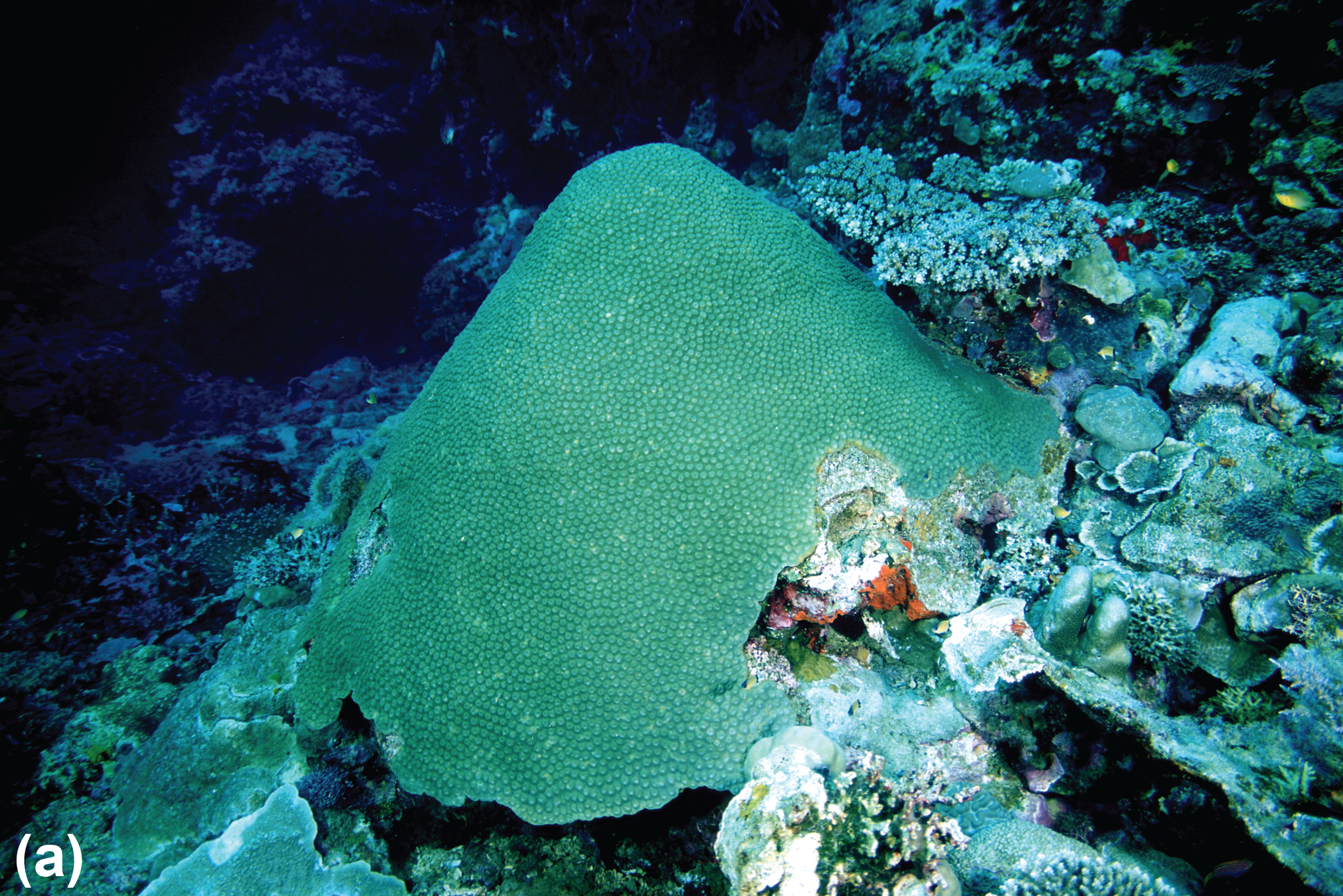
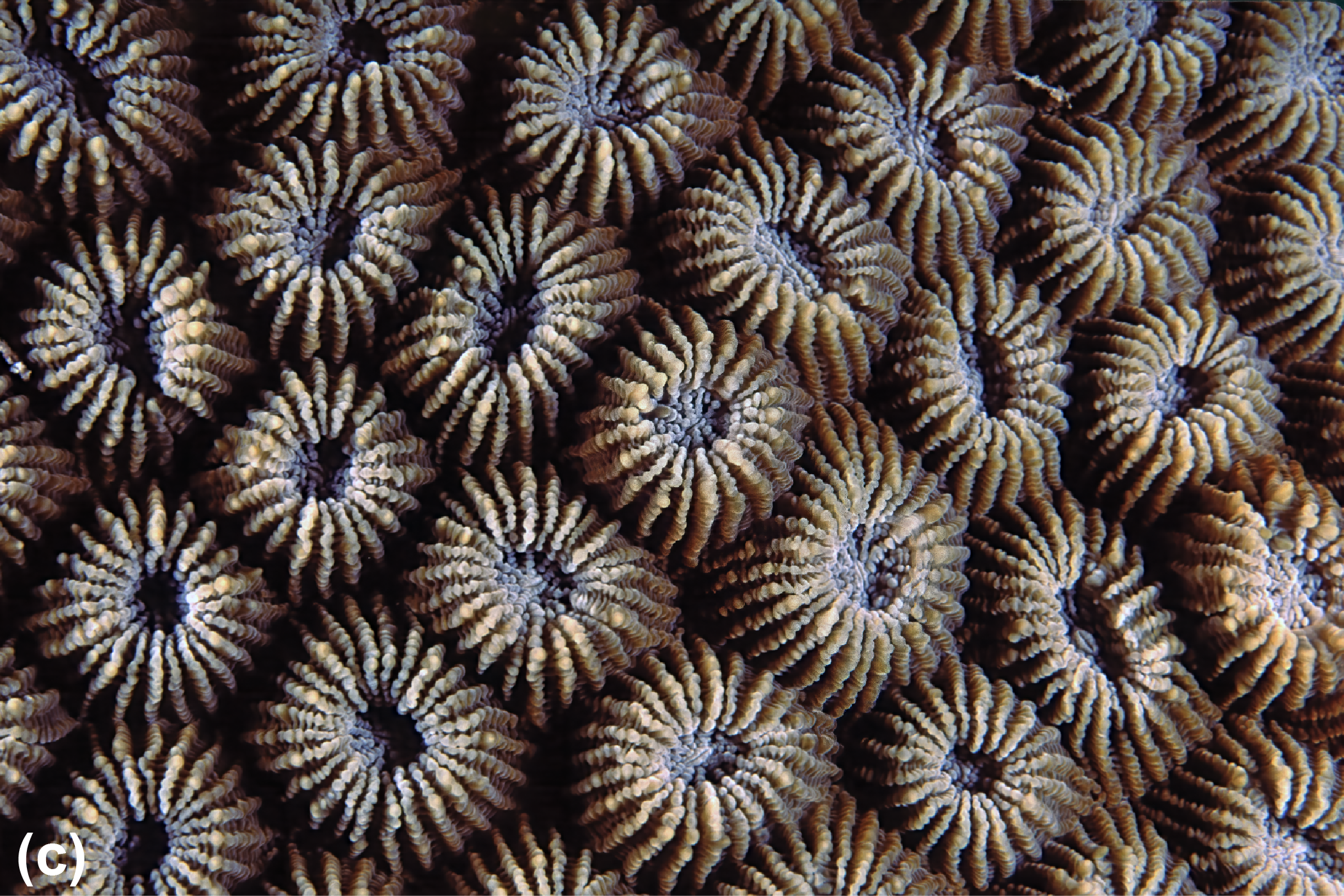
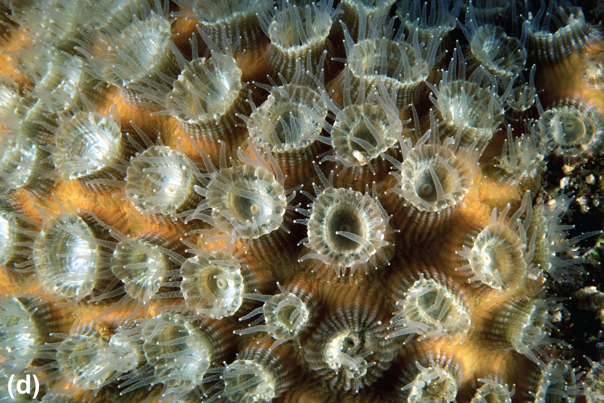
Although productivity is nutrient-limited throughout the tropical oceans, most coastal areas are characterized by extremely rich and abundant coral reef communities, except where turbidity is high or salinity is variable because of runoff. Despite the extremely low nutrient concentrations in the water column above, the coral communities thrive as a result of a unique symbiotic relationship between algae and reef-building corals.

Reef-building corals consist of millions of individual tiny animals whose hard parts are cemented together to form the coral mass (Fig. 13-12). Each coral animal, or polyp, contains within its tissues a large number of dinoflagellate algae known as zooxanthellae. The relationship between coral and zooxanthellae is complex and not fully understood, but one of the principal effects of, or reasons for, this partnership is thought to be more efficient utilization of the small amounts of nutrients available in tropical waters. The zooxanthellae and coral polyps continuously and rapidly recycle nutrients between themselves, thus retaining these nutrients in the photic zone.

  

  

Figure 13-12. Reef-building corals. (a) A typical reef-building hard coral colony (probably Diploastrea heliopora, Papua New Guinea). (b) Another typical hard coral (possibly Pocillopora sp., Papua New Guinea). (c, d) Individual polyps of Diploastrea heliopora (Papua New Guinea) are photographed (c) during the day when the polys are not open, versus (d) during the night, when the polyps have extended their soft tentacles to feed on zooplankton or particles.

Reef-building corals can grow only in the photic zone, where their zooxanthellae can photosynthesize. Hence, these corals are present only in relatively shallow water. In high-turbidity regions, the depth of the photic zone is reduced and coral reef communities do not develop. Coral polyps are adversely affected by high concentrations of suspended particulates, as they have limited ability to remove particles that are deposited on them to avoid being smothered. The high turbidity associated with high particle concentrations also reduces the amount of light available for their zooxanthellae to photosynthesize. Thus, reef building corals die if high concentrations of suspended sediment are sustained. Increased turbidity due to human activities has destroyed or damaged many such coral reef communities (Chap. 16).

Mid-Latitudes

During winter in the mid-latitudes, cooling of surface waters and mixing by wind waves eliminate the seasonal thermocline and mix water that has high nutrient concentrations from below the thermocline into the mixed layer (Fig. 13-9c). Phytoplankton are distributed almost randomly throughout the mixed layer because of their limited swimming capabilities. Because the mixed layer is much deeper than the photic zone, phytoplankton are within the photic zone during only a small percentage of the time. Although they can still photosynthesize for some depth below the photic zone, they cannot photosynthesize enough to replace the biomass they use for respiration, and they must survive long enough to return to the surface layer for growth and reproduction to resume. Therefore, during winter, phytoplankton growth is light-limited, populations are low, and many species adopt a hibernation-like resting phase.

In spring, light intensity increases and the photic zone becomes deeper. At the same time, storms are reduced, surface waters begin to warm, the mixed-layer depth is reduced, and a seasonal thermocline begins to form. Phytoplankton are now in the photic zone for an increased percentage of their time, and nutrients remain plentiful. The phytoplankton begin to photosynthesize, grow, and reproduce rapidly.

The standing stock (biomass) of phytoplankton increases rapidly at the beginning of the spring bloom period, but the zooplankton population, which now has an increasing food supply, also begins to feed, grow, and reproduce rapidly. Consequently, the majority of new phytoplankton cells are eaten by zooplankton, and the rapid reproduction of phytoplankton does not lead to sustained high phytoplankton concentrations (Fig. 13-13). The standing stock of phytoplankton represents only a small percentage of the total production because many of them are lost to consumption by herbivores or to sinking.

Figure 13-13. During a phytoplankton bloom, such as the spring bloom in mid-latitudes, the production rate of new biomass by phytoplankton rises rapidly and is followed, with a time lag of a few days, by a similar increase in zooplankton production. The phytoplankton biomass (standing stock) increases somewhat during the early part of the bloom, but it is rapidly reduced by zooplankton feeding, even though the phytoplankton production rate continues to increase.

As spring continues, phytoplankton rapidly deplete nutrients in the mixed layer. In addition, the mixed layer becomes shallower (about 10 to 15 m) as the seasonal thermocline forms. At this time, the phytoplankton have adequate light but are nutrient-limited. Consequently, their growth slows and the spring bloom collapses as zooplankton continue to feed on them. Soon, the zooplankton population also declines as its food supply decreases, and the zooplankton continue to be eaten by their predators.

During summer, primary productivity continues at a low level, supported by nutrients recycled by the consumers and decomposers in the mixed layer. However, most of these nutrients are recycled below the seasonal thermocline, where light levels are too low to support significant phytoplankton growth.

In fall, cooling and winter storms again weaken the seasonal thermocline, and nutrients are mixed into the photic zone from waters below. The addition of nutrients often supports a fall bloom of phytoplankton. However, the photic zone is now shallower because of the declining light intensity. Variations in timing, location, and year-to-year climate are particularly important in determining the magnitude of the fall bloom. If nutrients are mixed into the surface layer before the light intensity declines too much and before the mixed layer becomes too deep, a fall bloom occurs. Fall blooms are generally smaller and of shorter duration than spring blooms. If the nutrients are not mixed into the surface layer until late fall, when light intensity is already very low, no fall bloom occurs. In addition, no fall bloom occurs if intense cooling or strong storms eliminate the seasonal thermocline early and create a continuously mixed, very deep mixed layer.

In early winter, the enhanced mixing by storm winds, surface water cooling, and declining light levels combine to return the system to its winter state, in which the phytoplankton are light-limited.

Each year, at each location, the seasonal phytoplankton cycle is different from that of the previous years because of variations in weather. In addition, the details of the cycle vary in response to other influences, such as the composition of planktonic species, and the concentrations of nutrients other than nitrogen and phosphorus (particularly the concentration of silicate). The subtle and complex interactions between ocean physics, chemistry, and biology that control the seasonal plankton cycle are further complicated in some coastal regions by other processes, such as the introduction of suspended sediment and nutrients by rivers and coastal upwelling.

Phytoplankton Species Succession 

Many herbivores are selective feeders that require or prefer certain characteristics in the phytoplankton they eat. Most commonly, the requirement or preference is that the food species be within a range of sizes suited to the animals’ feeding methods. Larger zooplankton and juvenile fishes generally require large phytoplankton cells that are easy to capture and provide larger amounts of food. Smaller zooplankton specialize in eating smaller phytoplankton. Most coastal food chains that lead to commercially valuable fish and shellfish species are short and based primarily on larger phytoplankton species that are eaten by zooplankton and juvenile fishes. Food chains based on the smaller phytoplankton species are generally longer and less efficient (CC15), and support fish and shellfish species of generally lesser commercial value. Microbial food chains may be short, but they are thought to be partially self-contained, with much of the organic matter produced being recycled by microbial species rather than consumed in food chains leading to commercially valuable species.

Many factors influence phytoplankton species composition, including temperature, salinity, light intensity, and nutrient concentrations. Because these factors vary seasonally, phytoplankton species composition also varies during the year in most locations. Many different species of phytoplankton are always present at any location, but one or, at most, a few species generally dominate and constitute the majority of phytoplankton. As environmental factors change, one dominant species is replaced by another in a progression called species succession.

Phytoplankton species succession can be highly complex and can vary, often greatly, from year to year. One species may become dominant at approximately the same time of year for many years, but may not become dominant at all in other years.

In high latitudes and in regions of persistent upwelling, nutrients are present in relatively high concentrations throughout the phytoplankton growth period. High nutrient concentrations favor larger phytoplankton species, which are predominantly diatoms. Diatoms dominate the phytoplankton community throughout the active growth period in these regions, which consequently support short, efficient food webs (CC15).

In mid-latitudes, nutrient concentrations vary during the summer growing period. In spring, nutrient concentrations are high, and, consequently, diatoms dominate. The spring bloom of diatoms removes most nutrients from the water column, causing the bloom to collapse and to be replaced by flagellates (Fig. 13-14). During summer, after the spring diatom bloom, flagellates (sometimes a succession of different species) dominate the phytoplankton community. The flagellates can obtain their nutrients from the very low concentrations that are sustained by nutrient recycling in the photic zone. In fall, storms return enough nutrients to the photic zone to support fall diatom blooms in some years and areas.

Figure 13-14. The seasonal variations of nitrogen, phosphorus, silicon, diatoms, flagellates, and zooplankton in the mid-latitude coastal oceans usually follow a similar pattern each year. The spring bloom of diatoms rapidly depletes the nutrients, and the diatoms are superseded by dinoflagellates. Because the dinoflagellates are not suitable food for many zooplankton species, the zooplankton population also declines. By utilizing nutrients recycled within the photic zone, flagellates and some diatoms continue primary production at relatively low levels throughout the summer. A fall bloom of diatoms often occurs when storms and cooling weaken the thermocline and return some nutrients to the surface layer by mixing. In late fall, the light intensity becomes too low to support substantial primary production. Thus, decomposition, cooling, and wind mixing enable the return of nutrients to the surface layer before the following spring.

As a result of the seasonal availability of diatoms, many species of zooplankton and juvenile fishes that prefer or require diatoms as food have life cycles that are attuned to the seasons. For example, some fish and invertebrate species spawn in spring, and their eggs hatch into larvae that feed voraciously on diatoms. The juvenile fishes reach a sufficient size by late spring, when the diatom bloom collapses, to be able to feed on zooplankton. Some species spawn twice during the year to take advantage of both spring and fall blooms.

Many mid-latitude fish and invertebrate species have life cycles that depend on the availability of abundant diatoms as food for their juveniles during only a few days or weeks at a specific time of year. However, the timing, intensity, and dominant species of seasonal diatom blooms vary from year to year. As a result, the survival rate of the larval stages of many fish and invertebrate species also varies from year to year. The number of juveniles that survive their first critical year of life is called the “year class strength.” Year class strength may be high if the species spawns at the optimal time and locations in relation to the seasonal phytoplankton cycle. If year-to-year variability causes spawning and the phytoplankton seasonal succession to be misaligned in time or location in any specific year, sufficient food is not available when needed and year class strength is low.

Phytoplankton species succession is further complicated by variations in the availability of specific nutrients, particularly silicate and nitrogen compounds. During the spring diatom bloom in the mid-latitudes, silicate may be depleted before other nutrients (Fig. 13-14), causing diatoms to be replaced by flagellates that do not require silica. Silica is recycled extremely slowly into solution once it has been incorporated in diatom frustules. As a result, silica is not returned to the photic zone until the fall, when nutrient-rich waters from below the seasonal thermocline are mixed back into the mixed layer. These deeper waters have relatively high concentrations of silica dissolved from diatom frustules and terrigenous particles.

All phytoplankton cells require and take up phosphorus and nitrogen in approximately the same ratio as these elements occur in seawater. Similarly, diatoms require and take up silica in a reasonably constant ratio to other nutrients. The proportions of silicate, phosphate, and nitrogen compounds in water below the permanent thermocline are remarkably constant throughout the oceans. In coastal regions, terrestrial runoff normally contains high concentrations of dissolved silicate.

Consider what might happen if there were an excess of nitrogen compounds and phosphate in relation to silicate at the onset of the spring diatom bloom. The diatom bloom would deplete silicate sooner than nitrogen and phosphorus. Flagellates would replace diatoms and could bloom explosively because nitrogen and phosphorus would still be ample. This bloom might produce very large standing stocks of flagellates if, as is often true, herbivores that are able to graze the tiny flagellate cells efficiently were not abundant and could not reproduce quickly. Flagellate blooms do occur periodically, although infrequently, in limited regions where runoff has high nitrogen and phosphorus concentrations but low silicate concentrations. Blooms are becoming more frequent and widespread in regions near centers of human population, particularly where coastal waters have long residence times. Some of these blooms are caused by or substantially strengthened by the huge volumes of treated or untreated human sewage wastes and agricultural fertilizer discharged to the oceans (Chap. 16). Untreated sewage has high concentrations of nitrogen compounds and phosphate but relatively low silicate concentrations and sewage treatment employed in most locations in the U.S. and worldwide does not remove nitrogen or phosphorus.