4.3: Turbulent Flow in Channels - Initial Material
- Page ID
- 4171
\( \newcommand{\vecs}[1]{\overset { \scriptstyle \rightharpoonup} {\mathbf{#1}} } \)
\( \newcommand{\vecd}[1]{\overset{-\!-\!\rightharpoonup}{\vphantom{a}\smash {#1}}} \)
\( \newcommand{\id}{\mathrm{id}}\) \( \newcommand{\Span}{\mathrm{span}}\)
( \newcommand{\kernel}{\mathrm{null}\,}\) \( \newcommand{\range}{\mathrm{range}\,}\)
\( \newcommand{\RealPart}{\mathrm{Re}}\) \( \newcommand{\ImaginaryPart}{\mathrm{Im}}\)
\( \newcommand{\Argument}{\mathrm{Arg}}\) \( \newcommand{\norm}[1]{\| #1 \|}\)
\( \newcommand{\inner}[2]{\langle #1, #2 \rangle}\)
\( \newcommand{\Span}{\mathrm{span}}\)
\( \newcommand{\id}{\mathrm{id}}\)
\( \newcommand{\Span}{\mathrm{span}}\)
\( \newcommand{\kernel}{\mathrm{null}\,}\)
\( \newcommand{\range}{\mathrm{range}\,}\)
\( \newcommand{\RealPart}{\mathrm{Re}}\)
\( \newcommand{\ImaginaryPart}{\mathrm{Im}}\)
\( \newcommand{\Argument}{\mathrm{Arg}}\)
\( \newcommand{\norm}[1]{\| #1 \|}\)
\( \newcommand{\inner}[2]{\langle #1, #2 \rangle}\)
\( \newcommand{\Span}{\mathrm{span}}\) \( \newcommand{\AA}{\unicode[.8,0]{x212B}}\)
\( \newcommand{\vectorA}[1]{\vec{#1}} % arrow\)
\( \newcommand{\vectorAt}[1]{\vec{\text{#1}}} % arrow\)
\( \newcommand{\vectorB}[1]{\overset { \scriptstyle \rightharpoonup} {\mathbf{#1}} } \)
\( \newcommand{\vectorC}[1]{\textbf{#1}} \)
\( \newcommand{\vectorD}[1]{\overrightarrow{#1}} \)
\( \newcommand{\vectorDt}[1]{\overrightarrow{\text{#1}}} \)
\( \newcommand{\vectE}[1]{\overset{-\!-\!\rightharpoonup}{\vphantom{a}\smash{\mathbf {#1}}}} \)
\( \newcommand{\vecs}[1]{\overset { \scriptstyle \rightharpoonup} {\mathbf{#1}} } \)
\( \newcommand{\vecd}[1]{\overset{-\!-\!\rightharpoonup}{\vphantom{a}\smash {#1}}} \)
\(\newcommand{\avec}{\mathbf a}\) \(\newcommand{\bvec}{\mathbf b}\) \(\newcommand{\cvec}{\mathbf c}\) \(\newcommand{\dvec}{\mathbf d}\) \(\newcommand{\dtil}{\widetilde{\mathbf d}}\) \(\newcommand{\evec}{\mathbf e}\) \(\newcommand{\fvec}{\mathbf f}\) \(\newcommand{\nvec}{\mathbf n}\) \(\newcommand{\pvec}{\mathbf p}\) \(\newcommand{\qvec}{\mathbf q}\) \(\newcommand{\svec}{\mathbf s}\) \(\newcommand{\tvec}{\mathbf t}\) \(\newcommand{\uvec}{\mathbf u}\) \(\newcommand{\vvec}{\mathbf v}\) \(\newcommand{\wvec}{\mathbf w}\) \(\newcommand{\xvec}{\mathbf x}\) \(\newcommand{\yvec}{\mathbf y}\) \(\newcommand{\zvec}{\mathbf z}\) \(\newcommand{\rvec}{\mathbf r}\) \(\newcommand{\mvec}{\mathbf m}\) \(\newcommand{\zerovec}{\mathbf 0}\) \(\newcommand{\onevec}{\mathbf 1}\) \(\newcommand{\real}{\mathbb R}\) \(\newcommand{\twovec}[2]{\left[\begin{array}{r}#1 \\ #2 \end{array}\right]}\) \(\newcommand{\ctwovec}[2]{\left[\begin{array}{c}#1 \\ #2 \end{array}\right]}\) \(\newcommand{\threevec}[3]{\left[\begin{array}{r}#1 \\ #2 \\ #3 \end{array}\right]}\) \(\newcommand{\cthreevec}[3]{\left[\begin{array}{c}#1 \\ #2 \\ #3 \end{array}\right]}\) \(\newcommand{\fourvec}[4]{\left[\begin{array}{r}#1 \\ #2 \\ #3 \\ #4 \end{array}\right]}\) \(\newcommand{\cfourvec}[4]{\left[\begin{array}{c}#1 \\ #2 \\ #3 \\ #4 \end{array}\right]}\) \(\newcommand{\fivevec}[5]{\left[\begin{array}{r}#1 \\ #2 \\ #3 \\ #4 \\ #5 \\ \end{array}\right]}\) \(\newcommand{\cfivevec}[5]{\left[\begin{array}{c}#1 \\ #2 \\ #3 \\ #4 \\ #5 \\ \end{array}\right]}\) \(\newcommand{\mattwo}[4]{\left[\begin{array}{rr}#1 \amp #2 \\ #3 \amp #4 \\ \end{array}\right]}\) \(\newcommand{\laspan}[1]{\text{Span}\{#1\}}\) \(\newcommand{\bcal}{\cal B}\) \(\newcommand{\ccal}{\cal C}\) \(\newcommand{\scal}{\cal S}\) \(\newcommand{\wcal}{\cal W}\) \(\newcommand{\ecal}{\cal E}\) \(\newcommand{\coords}[2]{\left\{#1\right\}_{#2}}\) \(\newcommand{\gray}[1]{\color{gray}{#1}}\) \(\newcommand{\lgray}[1]{\color{lightgray}{#1}}\) \(\newcommand{\rank}{\operatorname{rank}}\) \(\newcommand{\row}{\text{Row}}\) \(\newcommand{\col}{\text{Col}}\) \(\renewcommand{\row}{\text{Row}}\) \(\newcommand{\nul}{\text{Nul}}\) \(\newcommand{\var}{\text{Var}}\) \(\newcommand{\corr}{\text{corr}}\) \(\newcommand{\len}[1]{\left|#1\right|}\) \(\newcommand{\bbar}{\overline{\bvec}}\) \(\newcommand{\bhat}{\widehat{\bvec}}\) \(\newcommand{\bperp}{\bvec^\perp}\) \(\newcommand{\xhat}{\widehat{\xvec}}\) \(\newcommand{\vhat}{\widehat{\vvec}}\) \(\newcommand{\uhat}{\widehat{\uvec}}\) \(\newcommand{\what}{\widehat{\wvec}}\) \(\newcommand{\Sighat}{\widehat{\Sigma}}\) \(\newcommand{\lt}{<}\) \(\newcommand{\gt}{>}\) \(\newcommand{\amp}{&}\) \(\definecolor{fillinmathshade}{gray}{0.9}\)The big question at this point is this: how applicable to real flows are the equations for the distribution of shear stress and velocity in steady uniform flows in circular pipes and open channels derived in the preceding section? If you made experiments with pipe flows and channel flows at very low Reynolds numbers, before the transition to turbulent flow (remember, this would necessitate combinations of low velocities, high viscosities, and small flow depths and diameters), you would find beautiful agreement between theory and observation—something that is always satisfying for both the theoretician and the experimentalist. But for turbulent flows, which is the situation in most flows that are of practical interest, the story is different.
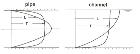
Figure \(\PageIndex{1}\) shows a comparison of velocity profiles, in both pipes and channels, between laminar and turbulent flows arranged to have the same discharge. It is clear that the turbulent-flow velocity profiles are much more nearly uniform over most of the flow but show a much sharper change in velocity near the boundary, where by the no-slip condition the velocity has to go to zero. It is easy to understand qualitatively why this is so: the exchange of turbulent eddies—macroscopic masses or parcels of fluid—across the surfaces of mean shearing normal to the solid boundaries is much better at ironing out cross-flow velocity differences than is just the exchange of molecules over short distances in laminar flow. But then the velocity gradient near the boundary, where the normal-to-boundary motions of eddies are inhibited by the presence of the boundary itself, must be even sharper than in laminar flow.

The story with shear stress is different. If you look back at the derivation of Equation 4.2.4 for the shear-stress distribution in a channel flow, there is nothing in the underlying assumptions that is specific to laminar flow, so the results—the linear distribution of shear stress—should hold just as well in turbulent flow as in laminar flow. I will be making use of that fact later in this chapter.
You might be tempted to ask why Equation 4.2.7 breaks down for turbulent flow. The most straightforward answer (although not the most important) is, with reference to the channel flow, that we can no longer assume that the shear stress across planes in the flow parallel to the bottom boundary is given by Equation 1.3.6, \(\tau=\mu(d u / d y)\), so we can no longer eliminate \(\tau\) and perform the integration as in Equation 4.2.7.
Now to get down to more important reasons: part of the reason Equation 4.2.7 is no longer applicable is simply that on account of the irregularity of the fluid motion in the turbulent case the surfaces of local shear are oriented differently at each point on such a plane, and the rate or intensity of shear varies as well. But there is a more important reason that has to do with the basic nature of shear stress in turbulent flow past a solid boundary, which I will deal with in the next section. Suffice it to say here that in one important sense the viscosity is effectively much greater in turbulent flows, again because of the efficacy with which turbulent eddies transport fluid momentum across planes of mean shearing; remember that the basic nature of viscosity itself arises from such momentum exchange on the part of the constituent molecules of the fluid.
This inability to obtain a theoretical velocity distribution in turbulent flows is just one example of a general problem with such flows: it is not possible to solve the equations of motion to obtain exact solutions. The reason for this is basically similar to, although more general than, the problem with velocity profiles noted above: we know what equations we have to solve but we cannot solve them because of the uncertainty that turbulence introduces into the application of these equations. The great number of equations to be found in textbooks and papers on turbulent flow are semi-empirical: the general form of the equation may be suggested by physical reasoning, but the numerical constants in the equation, and therefore its specific form, must be found from experiments. And in many cases not even the general form of the equation is known, and the curve must be obtained entirely by experiment. This should become abundantly clear in the material on resistance and velocity profiles in turbulent flow below.


