4.4: Turbulent Shear Stress

One of the most significant effects of turbulence is the transport of such things as heat, momentum, solute, or suspended matter—material or properties that can be viewed as carried passively by the fluid—across planes parallel to the mean flow by the random motions of fluid masses back and forth across these planes. The mean normal-to-boundary velocity across such planes is by definition zero, so the net mass of fluid transferred back and forth in this way must balance to zero on the average. But if the material or property passively associated with the fluid is on the average unevenly distributed—if its average value varies in a direction normal to the mean motion—then the balanced turbulent transfer of fluid across the planes causes a diffusive transport or “flow” of this property, usually referred to as a flux, in the direction of decreasing average value. This kind of transport is called turbulent diffusion.

To see the turbulent diffusion of some material or property carried by the fluid, think about the result of an exchange of two fluid parcels or eddies with equal mass across a plane of mean shear parallel to the boundary in a turbulent boundary layer (Figure \(\PageIndex{1}\)). The eddy traveling from the side of the plane with higher average value of some property \(\text{P}\) tends to arrive on the other side with a higher value of \(\text{P}\) than its new surroundings, and conversely the eddy traveling from the side with lower average value tends to arrive with a lower value than its surroundings. The exchange thus tends to even out the distribution of \(\text{P}\) by means of a net transport of \(\text{P}\) in the direction of decreasing average value.

Figure \(\PageIndex{1}\): Transport of a material or a property by turbulent diffusion in a turbulent boundary layer.

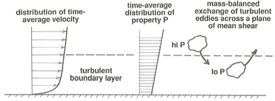
An irregular or nonuniform distribution of the property \(\text{P}\) at the scale of individual eddies is to be expected by the very nature of the diffusion process. So not every eddy that crosses the plane of mean shear shown in Figure \(\PageIndex{1}\) from the side with higher average \(\text{P}\) arrives on the other side with a value of \(\text{P}\) higher than the new surroundings, and conversely not every eddy crossing in the other direction arrives with a lower value of \(\text{P}\). But the important point is that there is a tendency for this to happen because there is a statistical correlation between values of \(\text{P}\) and position normal to the plane, and therefore an average gradient of \(\text{P}\) in that direction. That average gradient is maintained by some process unrelated to diffusion.

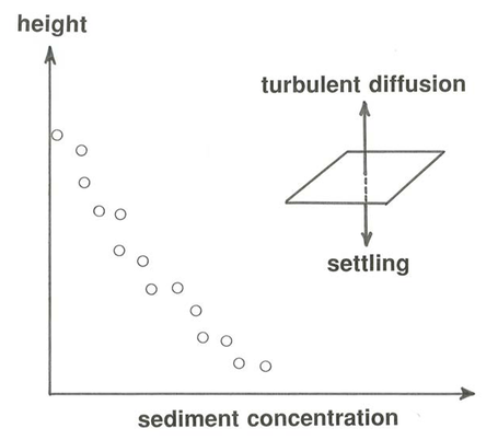
A simple but important example is that of sediment carried in suspension by a river or a tidal current or the atmosphere. (We will look at this problem in more detail in Part II.) You know that if a fluid flow is strong enough it can pick up particles of sand or dust from the lower boundary of the flow and carry them high up into the flow, whence they eventually settle back to the bed or the ground. The concentration of the suspended sediment decreases upward, because of the tendency of the sediment to settle through its surrounding fluid. There is a balance between downward settling and upward turbulent diffusion along the concentration gradient (Figure \(\PageIndex{2}\)). The correlation between suspended-sediment concentration and distance above the bottom is clear in Figure \(\PageIndex{2}\).

Figure \(\PageIndex{2}\): Balance between upward transport of suspended sediment by turbulent diffusion and downward transport by settling.

We can appeal to the idea of diffusion of fluid momentum to account for the differences in velocity distribution in laminar and turbulent flow down an inclined plane, discussed in an earlier section of this chapter. In laminar flow there are no eddies to be exchanged across shear planes parallel to the bottom, but the molecules themselves hurtle or weave randomly back and forth across these planes in loose analogy with the picture outlined above for the random motions of turbulent eddies. Because on average the molecules have a greater downchannel velocity in the region above a given shear plane than below it, molecular exchange across the plane tends to even out the distribution of fluid momentum and therefore also of fluid velocity. Fluid momentum is continuously created, by either the downslope forces of gravity or a driving downstream pressure gradient (or a combination of the two), then transported toward the bottom boundary by molecular diffusion, and in the process is “consumed” by the resistance force at the bottom boundary.

The tendency for molecular motions to even out the velocity distribution in a sheared fluid is in part the physical cause of the resistance of a fluid to shearing. In liquids the effect of transient molecular attractions in resisting shear is more important, but in gases the diffusive effect is the dominant one. The viscosity of a fluid is simply a measure of the effectiveness of molecular motions and/or molecular attractions in smoothing out an uneven velocity distribution or in maintaining the velocity distribution against the tendency for the fluid to accelerate downslope and intensify the shearing. The continuum hypothesis allows us to disregard the details of molecular forces and diffusion and regard the resulting shear stress as a point quantity.

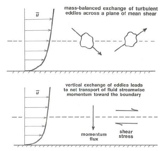
In turbulent flow, on the other hand, there is an additional diffusional mechanism for transport of fluid momentum toward the boundary: exchange of macroscopic fluid eddies across the planes of mean shear parallel to the bottom tends to even out the velocity distribution by diffusion of momentum toward the bottom (Figure \(\PageIndex{3}\)). By Newton’s second law this rate of transport of momentum by turbulent motions is equivalent to a shear stress across the plane. This is called the turbulent shear stress or, usually, the Reynolds stress. It has exactly the same physical effect as an actual frictional force exerted directly between the two layers of fluid on either side of the plane: the faster-moving fluid above the plane exerts an accelerating force on the slower-moving fluid below the plane, and conversely the fluid below exerts an equal and opposite retarding force on the fluid above. It is true that the “range of operation” of this force is smeared out indefinitely for some distance on either side of the plane, but the result is the same as that of a force exerted directly across the plane.

Figure \(\PageIndex{3}\): The origin of turbulent shear stress.

The total shear stress across a shear plane in the flow is the sum of the turbulent shear stress, caused by macroscopic diffusion of fluid momentum, and the viscous shear stress, caused in part by molecular diffusion of fluid momentum and in part by attractive forces between molecules at the shear plane. Owing to its macroscopic nature the turbulent shear stress can be associated with a given point on a shear plane only in a formal way; the viscous shear stress, although it has real physical meaning from point to point, must be regarded as an average over the area of the shear plane, because in turbulent flow both the magnitude and the orientation of shearing vary (continuously, and on the scale of eddies) from point to point.

In an earlier section of this chapter we derived expressions (Equation 4.2.3) for the shear stress across shear planes in laminar flow in a pipe or a channel. The shear stress in those two equations is the sum of the turbulent shear stress and the viscous shear stress. You may protest that the results in Equation 4.2.3 was obtained for laminar flow only. But in deriving the equations we did not assume anything at all about the internal nature of the flow, only that the flow is steady and uniform on the average. This is in contrast to the results for velocity distribution, Equation 4.2.7, which involve the assumption that the shear stress across a shear plane is given by Equation 1.3.6, an assumption that is inadmissible for turbulent flow because of the importance of the additional turbulent shear stress. The linear distribution of shear stress from zero at the surface to a maximum at the bottom should therefore hold just as well for turbulent flow as for laminar flow, provided only that the flow is steady and uniform on average.

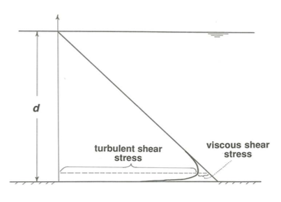
Except very near the solid boundary, where the normal-to- boundary component of the turbulent velocity must go to zero, the turbulent shear stress is far greater than the viscous shear stress. This is because turbulent exchange of fluid masses acts on a much larger scale than the molecular motions involved in the viscous shear stress and therefore transports momentum much more efficiently. Figure \(\PageIndex{4}\) is a plot of the distribution of turbulent shear stress and viscous shear stress in steady uniform flow down a plane. The total shear stress is given by the straight line, and the turbulent shear stress is given by the curve that is almost coincident with the straight line all the way from the surface to very near the bottom but then breaks sharply away to become zero right at the bottom. The difference between the straight line for total shear stress and the curve for turbulent shear stress represents the viscous shear stress; this is important only very near the boundary.

Figure \(\PageIndex{4}\): Distribution of total shear stress, turbulent shear stress, and viscous shear stress in a steady and uniform open-channel flow.

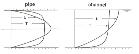
Because the turbulent shear stress is so much larger than the viscous shear stress except very near the boundary, differences in time- average velocity from layer to layer in turbulent flow are much more effectively ironed out over most of the flow depth than in laminar flow. This accounts for the much gentler velocity gradient \(du/dy\) over most of the flow depth in turbulent flow than in laminar flow; go back and look at Figure 4.3.1. But as a consequence of this gentle velocity gradient over most of the flow depth, near the bottom boundary, where viscous effects rather than turbulent effects are dominant, the velocity gradient is much steeper than in laminar flow, because the shearing necessitated by the transition from the still-large velocity near the boundary to the zero velocity at the boundary (remember the no-slip condition) is compressed into a thin layer immediately adjacent to the boundary.

Turbulence Closure Problem

When the Navier–Stokes equations are written for turbulent flow, and then instantaneous velocities are converted to their mean and fluctuating components, as was done in Chapter 3, time averages of products of fluctuating quantities (the Reynolds stresses mentioned in the previous section) emerge as new unknowns—and when one tries to characterize those new unknowns, further new unknowns arise! The result is that the equations of motion for turbulent flow can never form a closed system in which the number of equations is equal to the number of unknowns. This is called the turbulence closure problem. It is often said to be one of the great unsolved problems in all of physics. (That is a very strong statement.)

Various strategies have been devised to circumvent the closure problem, by making certain assumptions or parameterizations. A simple and widely used example must suffice here: parameterizing the nature of turbulent momentum transport in a turbulent shear flow by use of the eddy viscosity, and how it varies from the boundary of the flow into the interior.