3.8.2: Amphidromic Systems

The propagation of the tide is influenced by friction and resonances determined by the shapes and depths of the ocean basins and marginal seas. Because of the large scale of the tidal motion, the tidal propagation is also influenced by Coriolis acceleration (see Intermezzo 3.1). Generally we can neglect the effect of Coriolis for waves shorter than a few kilometres. In the previous section we found tidal wavelengths of the order of thousands of kilometres in the oceans and of the order of hundreds of kilometres in shallow seas.

Figure 3.28: Normal standing wave.

Figure 3.29: Tidal oscillation of a basin (Northern Hemisphere). The frequency of the oscillation is determined by the size of the basin and its depth.

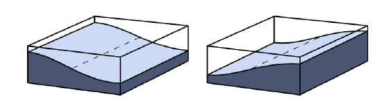
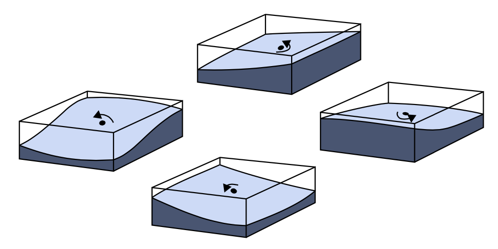
Since the movement of the tides is deflected by Coriolis and blocked by land masses, rotary movements are formed in oceans basins, bays and seas that are counter-clockwise in the Northern Hemisphere and clockwise in the Southern Hemisphere. Such rotary systems are called amphidromic systems. In an amphidromic system the wave progresses about a node (no vertical displacement) with the antinodes (maximum vertical displacement) rotating about the basin’s edges (see Figs. 3.28 and 3.29). The water can be seen to be sloshing around the basin. The node, where the amplitude of the vertical tide is zero, is called an amphidromic point.

Figure 3.30: Propagation of the \(M2\) tide in the Atlantic Ocean. The solid lines are co-tidal lines of simultaneous HW, the dashed line are the co-range lines of equal tidal range. Model results obtained using the FES2014 tide model. FES2014 was produced by Noveltis, Legos and CLS and distributed by Aviso +, with support from CNES (https://www.aviso.altimetry.fr/).

Figure 3.31: Propagation of the \(M2\) tide in the North Sea with co-tidal lines radiating away from the amphidromic points and co-range lines encircling them. The co-tidal lines show that the phase increases counter-clockwise around the amphidromic point (typical of NH amphidromes). The co-range lines show the tidal range increasing away from the node. Model results obtained using the FES2014 tide model. FES2014 was produced by Noveltis, Legos and CLS and distributed by Aviso+, with support from CNES (https://www.aviso.altimetry.fr/).

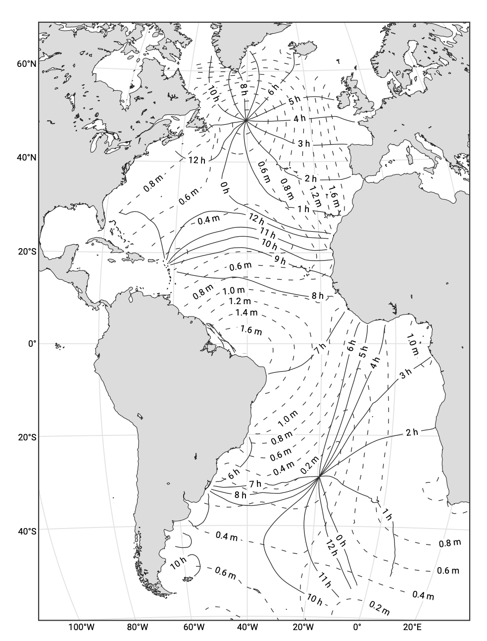
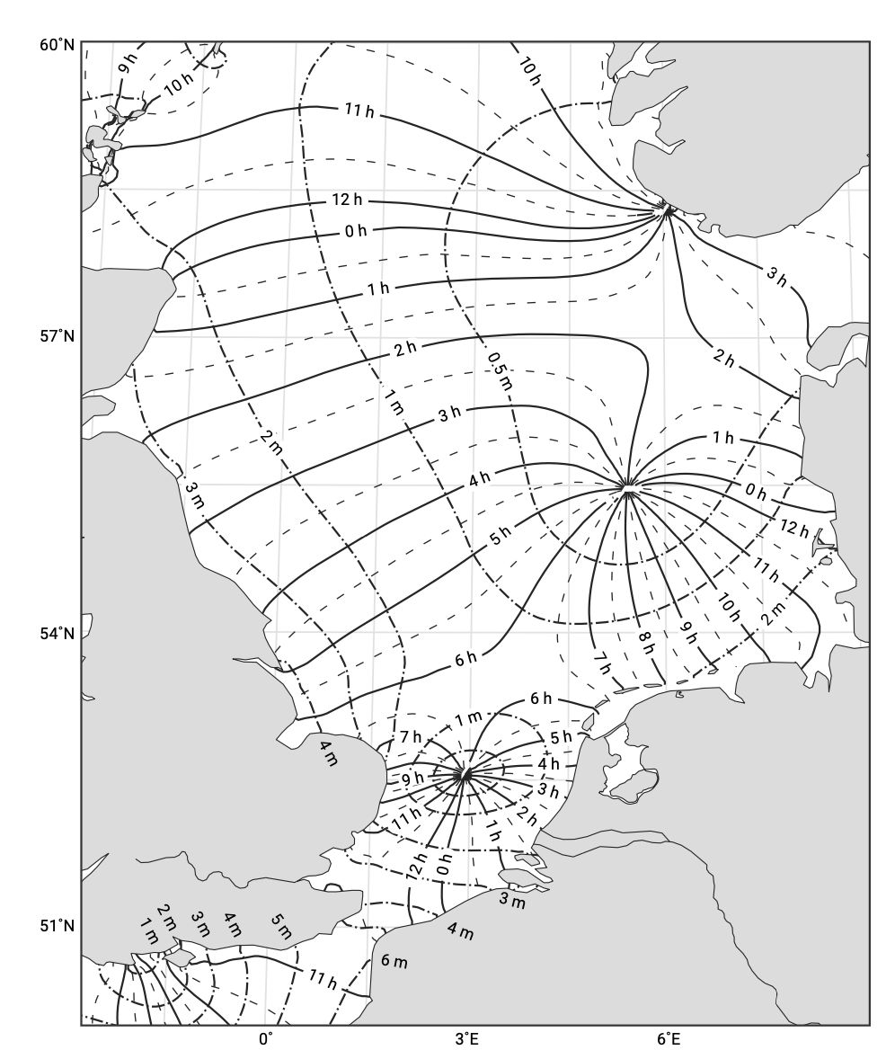
It is possible to visualise the propagation of the tidal wave by mapping the lines of simultaneous high water (occurrence of High Water (HW) in sun hours after moon culmination) and the lines of equal tidal range (vertical distance between HW and Low Water (LW) in m). The lines of simultaneous HW are called co-tidal lines or, since these lines connect points of equal phase, co-phase lines. They often radiate away from a node and are not equally spaced, since the propagation speed depends on the water depth h. Co-range lines connect points experiencing the same tidal range. They often form irregular concentric circles about a node. This is illustrated in Fig. 3.30 and Fig. 3.31.

An amphidromic point is said to be degenerate when its centre appears to be located over land rather than water. Examples are found at the southern tip of Norway and northwest of Bournemouth (along the southwest coast of England, southeast of Bristol, see Fig. 3.31).

Evidently, the local tide at a coastal location is dependent on the size, shape and depth of the basin. Every place along the coasts of the world has its own specific tidal curve. If the tidal forcing is in resonance with an oscillation period for the sea or bay, the tidal range is amplified and can be enormous. At some locations, the difference between high and low water is up to 12 m (compare that to the few decimetres at the open oceans!).