21.5: Gaia Hypothesis and Daisyworld

James Lovelock proposed a thought-provoking hypothesis: life regulates the climate to create an environment that favors life. Such self-maintained stability is called homeostasis. His hypothesis is called gaia — Greek for “mother Earth”.

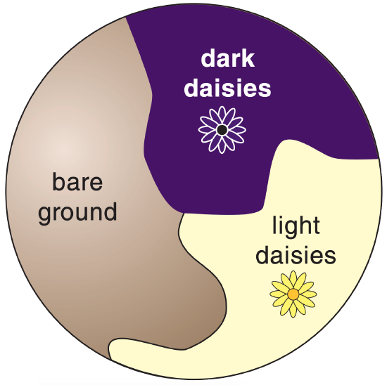
Lovelock and Andrew Watson illustrate the “biological homeostasis of the global environment” with daisyworld, a hypothetical Earth containing only light and dark colored daisies. If the Earth is too cold, the dark daisies proliferate, increasing the absorption of solar radiation. If too warm, light-colored daisies proliferate, reflecting more sunlight by increasing the global albedo (Fig. 21.22).

Figure 21.22 A hypothetical daisyworld with only light and dark colored flowers and bare ground.

21.5.1. Physical Approximations

We modify Lovelock’s toy model here to enable an easy solution of daisyworld on a spreadsheet. Given are two constants: the Stefan-Boltzmann constant σ_SB = 5.67x10^–8 W·m^–2·K^–4 and solar irradiance S_o = 1361 W·m^–2. Small variations in solar output are parameterized by luminosity, L , where L = 1 corresponds to the actual value for Earth. These factors are combined into a solar-forcing ratio, q:

\begin{align}q=\dfrac{L \cdot S_{o}}{4 \cdot \sigma_{S B}}\tag{21.40}\end{align}

The model forecasts the fraction of the globe covered by light daisies (C_L) and the fraction covered by dark daisies (C_D). Some locations will have no daisies, so the bare-ground fraction (C_G) of Earth’s surface is thus:

\begin{align}C_{G}=1-C_{D}-C_{L}\tag{21.41}\end{align}

To start the calculation, assume an initial state of C_L = C_D = 0.

Define a planetary albedo (A) as the coverage-weighted average of the individual daisy albedoes (A_i , which are adjustable parameters):

\begin{align}A=C_{G} \cdot A_{G}+C_{D} \cdot A_{D}+C_{L} \cdot A_{L}\tag{21.42}\end{align}

For this example, let:

A_L = 0.75 is the albedo of light-colored daisies

A_D = 0.25 is the albedo of dark-colored daisies

A_G = 0.5 is the bare-ground albedo (no flowers).

Use the planetary albedo with the solar forcing ratio to find daisyworld’s effective-radiation absolute temperature:

\begin{align}T_{e}^{4}=q \cdot(1-A)\tag{21.43}\end{align}

For a one-layer atmosphere with no window, the average surface temperature is

\begin{align}T_{s}^{4}=2 \cdot T_{e}^{4}\tag{21.44}\end{align}

Let Tr = 0.6 be an efficiency for horizontal heat transport. For example, Tr = 1 implies efficient spreading of heat around the globe, causing the local temperature to be controlled by the global-average albedo. Conversely, Tr = 0 forces the local temperature to be a function of only the local albedo in any one patch of daisies.

Thus, the patches of dark and light daisies have the following temperatures:

\begin{align}T_{D}^{4}=(1-T r) \cdot q \cdot\left(A-A_{D}\right)+T_{s}^{4}\tag{21.45a}\end{align}

\begin{align}T_{L}^{4}=(1-T r) \cdot q \cdot\left(A-A_{L}\right)+T_{s}^{4}\tag{21.45b}\end{align}

Suppose that daisies grow only if their patch temperatures are between 5°C and 40°C, and that daisies have the fastest growth rate (β) near the middle of this range (where T_o = 295.5 K = 22.5°C):

\begin{align}\beta_{D}=1-b \cdot\left(T_{o}-T_{D}\right)^{2}\tag{21.46a}\end{align}

\begin{align}\beta_{L}=1-b \cdot\left(T_{o}-T_{L}\right)^{2}\tag{21.46b}\end{align}

where negative values of β are truncated to zero. The growth factor is b = 0.003265 K^–2.

Because dark and light daisies interact via their change on the global surface temperature, you must iterate the coverage equations together as you step forward in time

\begin{align}C_{D \text { new }}=C_{D}+\Delta t \cdot C_{D} \cdot\left(C_{G} \cdot \beta_{D}-D\right)\tag{21.47a}\end{align}

\begin{align}C_{L \text { new }}=C_{L}+\Delta t \cdot C_{L} \cdot\left(C_{G} \cdot \beta_{L}-D\right)\tag{21.47b}\end{align}

where D = 0.3 is death rate (another adjustable parameter) for both light and dark daisies. In this iteration, the daisy coverages (C_D & C_L) at any one time step can be inserted into the right side of the above two equations, and the solution can be stepped forward in time to find the new coverages (C_{D new} & C_{L new}) one time step ∆t later. The time units are arbitrary, so you could use ∆t = 1 or ∆t = 0.5. To get daisies to grow if none are on the planet initially, assume a seed coverage of C_s = 0.01 and force C_{L new} ≥ C_s and C_{D new} ≥ C_s .

With the new coverages, eqs. (21.41 - 21.47) can be computed again for the next time step. Repeat for many time steps. For certain values of the parameters, the solution (i.e., coverages and temperatures) approaches a steady-state, which results in the desired homeostasis equilibrium.

21.5.2. Steady-state and Homeostasis

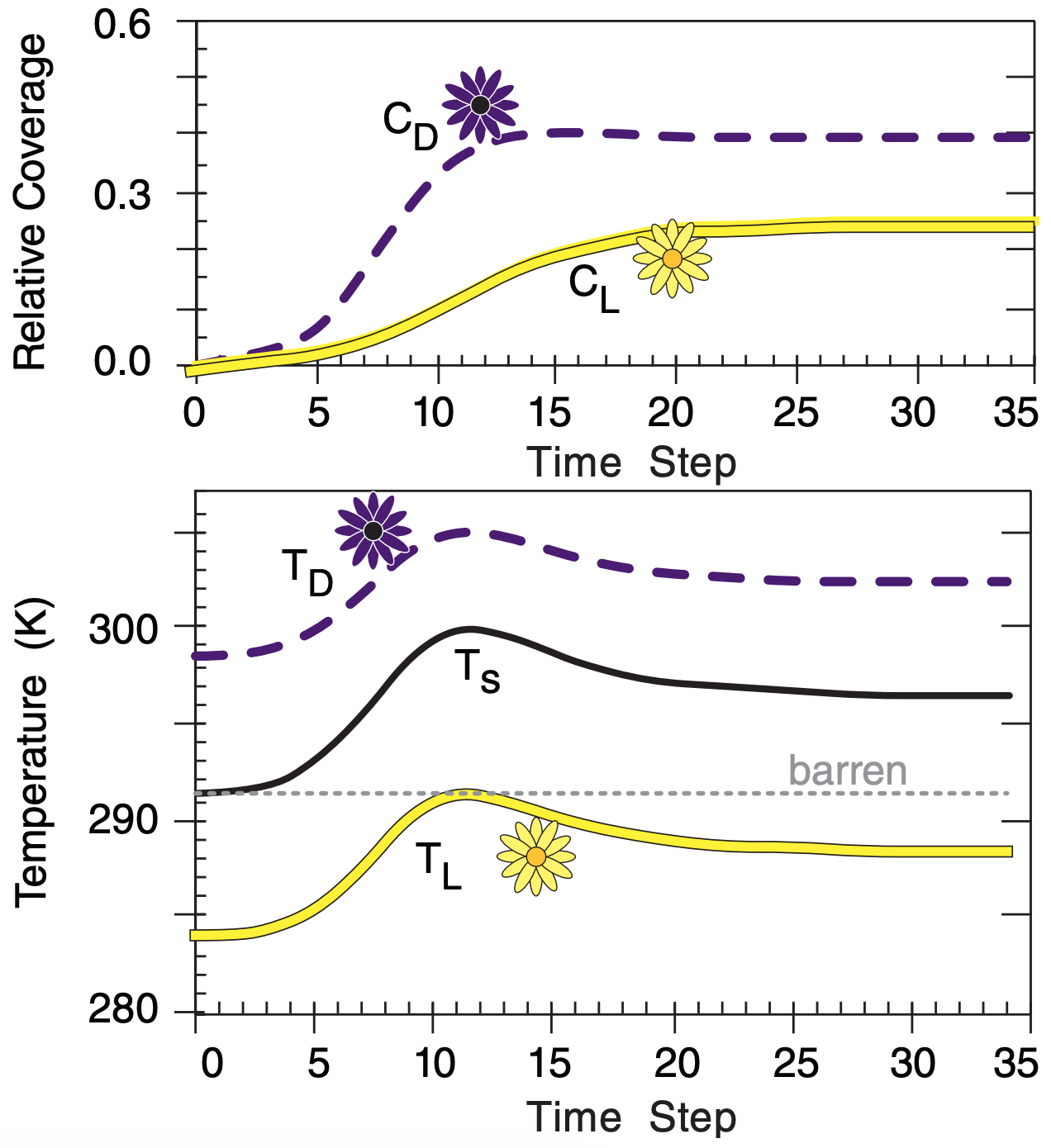
Suppose L = 1.2 with all other parameters set as described in the Physical Approximations subsection. After iterating, the final steady-state values are C_L = 0.24 , C_D = 0.40 and T_s = 296.8 K (see Fig. 21.23). Compare this to the surface temperature of a planet with no daisies: T_{s barren} = 291.3 K, found by setting A = A_G in eqs. (21.43 - 21.44).

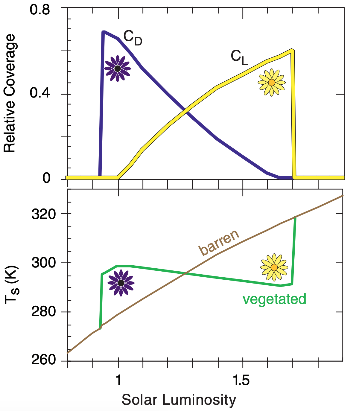
Suppose you rerun daisyworld with all the same parameters, but with different luminosity. The resulting steady-state conditions are shown in Fig. 21.24 for a variety of luminosities. For luminosities between about 0.94 to 1.70, the daisy coverage is able to adjust so as to maintain a somewhat constant Ts — namely, it achieves homeostasis. Weak incoming solar radiation (insolation) allows dark daisies to proliferate, which convert most of the insolation into heat. Strong insolation is compensated by increases in light daisies, which reflect the excess energy.

Figure 21.23 Evolution of daisy coverage and temperatures as daisyworld evolves toward an equilibrium, given a luminosity of L = 1.2 .

Figure 21.24 Final steady-state values of average surface temperature T_s and daisy coverages (C_D & C_L), as a function of luminosity. The bottom graph compares the lushly flowered (vegetated) world with an unflowered (barren) world.