
21.2: Astronomical Influences
- Page ID
- 10190

\( \newcommand{\vecs}[1]{\overset { \scriptstyle \rightharpoonup} {\mathbf{#1}} } \)
\( \newcommand{\vecd}[1]{\overset{-\!-\!\rightharpoonup}{\vphantom{a}\smash {#1}}} \)
\( \newcommand{\id}{\mathrm{id}}\) \( \newcommand{\Span}{\mathrm{span}}\)
( \newcommand{\kernel}{\mathrm{null}\,}\) \( \newcommand{\range}{\mathrm{range}\,}\)
\( \newcommand{\RealPart}{\mathrm{Re}}\) \( \newcommand{\ImaginaryPart}{\mathrm{Im}}\)
\( \newcommand{\Argument}{\mathrm{Arg}}\) \( \newcommand{\norm}[1]{\| #1 \|}\)
\( \newcommand{\inner}[2]{\langle #1, #2 \rangle}\)
\( \newcommand{\Span}{\mathrm{span}}\)
\( \newcommand{\id}{\mathrm{id}}\)
\( \newcommand{\Span}{\mathrm{span}}\)
\( \newcommand{\kernel}{\mathrm{null}\,}\)
\( \newcommand{\range}{\mathrm{range}\,}\)
\( \newcommand{\RealPart}{\mathrm{Re}}\)
\( \newcommand{\ImaginaryPart}{\mathrm{Im}}\)
\( \newcommand{\Argument}{\mathrm{Arg}}\)
\( \newcommand{\norm}[1]{\| #1 \|}\)
\( \newcommand{\inner}[2]{\langle #1, #2 \rangle}\)
\( \newcommand{\Span}{\mathrm{span}}\) \( \newcommand{\AA}{\unicode[.8,0]{x212B}}\)
\( \newcommand{\vectorA}[1]{\vec{#1}} % arrow\)
\( \newcommand{\vectorAt}[1]{\vec{\text{#1}}} % arrow\)
\( \newcommand{\vectorB}[1]{\overset { \scriptstyle \rightharpoonup} {\mathbf{#1}} } \)
\( \newcommand{\vectorC}[1]{\textbf{#1}} \)
\( \newcommand{\vectorD}[1]{\overrightarrow{#1}} \)
\( \newcommand{\vectorDt}[1]{\overrightarrow{\text{#1}}} \)
\( \newcommand{\vectE}[1]{\overset{-\!-\!\rightharpoonup}{\vphantom{a}\smash{\mathbf {#1}}}} \)
\( \newcommand{\vecs}[1]{\overset { \scriptstyle \rightharpoonup} {\mathbf{#1}} } \)
\( \newcommand{\vecd}[1]{\overset{-\!-\!\rightharpoonup}{\vphantom{a}\smash {#1}}} \)
\(\newcommand{\avec}{\mathbf a}\) \(\newcommand{\bvec}{\mathbf b}\) \(\newcommand{\cvec}{\mathbf c}\) \(\newcommand{\dvec}{\mathbf d}\) \(\newcommand{\dtil}{\widetilde{\mathbf d}}\) \(\newcommand{\evec}{\mathbf e}\) \(\newcommand{\fvec}{\mathbf f}\) \(\newcommand{\nvec}{\mathbf n}\) \(\newcommand{\pvec}{\mathbf p}\) \(\newcommand{\qvec}{\mathbf q}\) \(\newcommand{\svec}{\mathbf s}\) \(\newcommand{\tvec}{\mathbf t}\) \(\newcommand{\uvec}{\mathbf u}\) \(\newcommand{\vvec}{\mathbf v}\) \(\newcommand{\wvec}{\mathbf w}\) \(\newcommand{\xvec}{\mathbf x}\) \(\newcommand{\yvec}{\mathbf y}\) \(\newcommand{\zvec}{\mathbf z}\) \(\newcommand{\rvec}{\mathbf r}\) \(\newcommand{\mvec}{\mathbf m}\) \(\newcommand{\zerovec}{\mathbf 0}\) \(\newcommand{\onevec}{\mathbf 1}\) \(\newcommand{\real}{\mathbb R}\) \(\newcommand{\twovec}[2]{\left[\begin{array}{r}#1 \\ #2 \end{array}\right]}\) \(\newcommand{\ctwovec}[2]{\left[\begin{array}{c}#1 \\ #2 \end{array}\right]}\) \(\newcommand{\threevec}[3]{\left[\begin{array}{r}#1 \\ #2 \\ #3 \end{array}\right]}\) \(\newcommand{\cthreevec}[3]{\left[\begin{array}{c}#1 \\ #2 \\ #3 \end{array}\right]}\) \(\newcommand{\fourvec}[4]{\left[\begin{array}{r}#1 \\ #2 \\ #3 \\ #4 \end{array}\right]}\) \(\newcommand{\cfourvec}[4]{\left[\begin{array}{c}#1 \\ #2 \\ #3 \\ #4 \end{array}\right]}\) \(\newcommand{\fivevec}[5]{\left[\begin{array}{r}#1 \\ #2 \\ #3 \\ #4 \\ #5 \\ \end{array}\right]}\) \(\newcommand{\cfivevec}[5]{\left[\begin{array}{c}#1 \\ #2 \\ #3 \\ #4 \\ #5 \\ \end{array}\right]}\) \(\newcommand{\mattwo}[4]{\left[\begin{array}{rr}#1 \amp #2 \\ #3 \amp #4 \\ \end{array}\right]}\) \(\newcommand{\laspan}[1]{\text{Span}\{#1\}}\) \(\newcommand{\bcal}{\cal B}\) \(\newcommand{\ccal}{\cal C}\) \(\newcommand{\scal}{\cal S}\) \(\newcommand{\wcal}{\cal W}\) \(\newcommand{\ecal}{\cal E}\) \(\newcommand{\coords}[2]{\left\{#1\right\}_{#2}}\) \(\newcommand{\gray}[1]{\color{gray}{#1}}\) \(\newcommand{\lgray}[1]{\color{lightgray}{#1}}\) \(\newcommand{\rank}{\operatorname{rank}}\) \(\newcommand{\row}{\text{Row}}\) \(\newcommand{\col}{\text{Col}}\) \(\renewcommand{\row}{\text{Row}}\) \(\newcommand{\nul}{\text{Nul}}\) \(\newcommand{\var}{\text{Var}}\) \(\newcommand{\corr}{\text{corr}}\) \(\newcommand{\len}[1]{\left|#1\right|}\) \(\newcommand{\bbar}{\overline{\bvec}}\) \(\newcommand{\bhat}{\widehat{\bvec}}\) \(\newcommand{\bperp}{\bvec^\perp}\) \(\newcommand{\xhat}{\widehat{\xvec}}\) \(\newcommand{\vhat}{\widehat{\vvec}}\) \(\newcommand{\uhat}{\widehat{\uvec}}\) \(\newcommand{\what}{\widehat{\wvec}}\) \(\newcommand{\Sighat}{\widehat{\Sigma}}\) \(\newcommand{\lt}{<}\) \(\newcommand{\gt}{>}\) \(\newcommand{\amp}{&}\) \(\definecolor{fillinmathshade}{gray}{0.9}\)If the incoming solar radiation (insolation) changes, then the radiation budget of the Earth will adjust, possibly altering the climate. Two causes of daily-averaged insolation \(\ \overline{E}\) change at the top of the atmosphere are changes in solar output So and changes in Earth-sun distance R (recall eq. 2.21).
21.2.1. Milankovitch Theory
In the 1920s, astrophysicist Milutin Milankovitch proposed that slow fluctuations in the Earth’s orbit around the sun can change the sun-Earth distance. Distance changes alter insolation according to the inverse square law (eq. 2.16), thereby contributing to climate change. Ice-age recurrence (inferred from ice and sediment cores) was later found to be correlated with orbital characteristics, supporting his hypothesis. Milankovitch focused on three orbital characteristics: eccentricity, obliquity, and precession.
21.2.1.1. Eccentricity
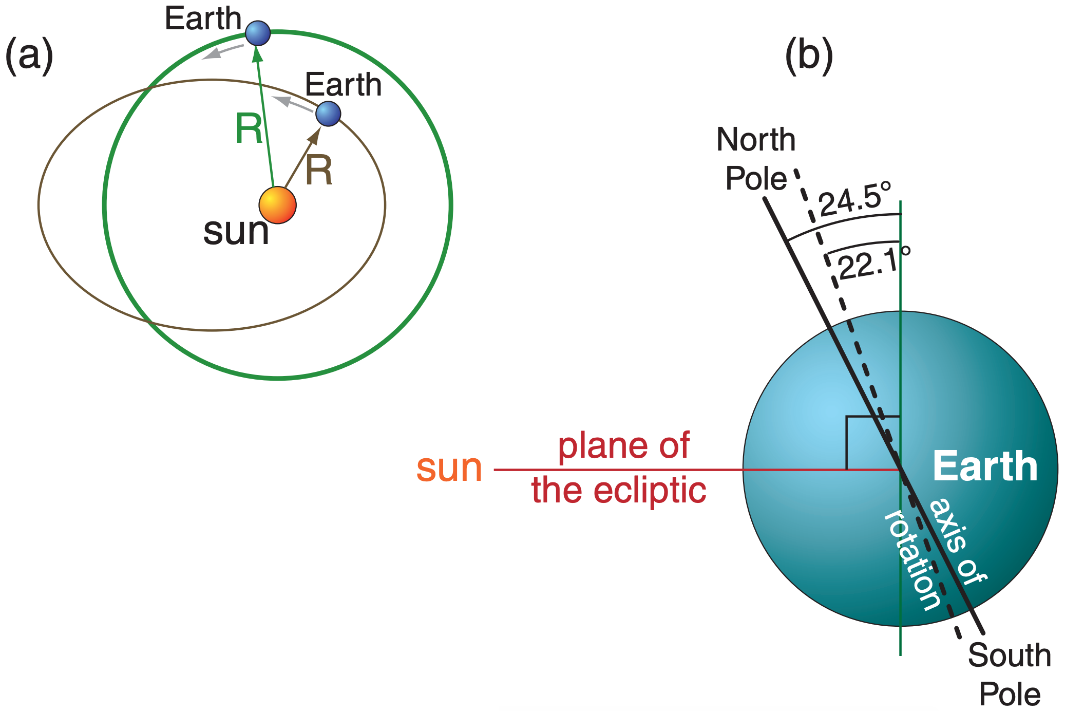
The shape of Earth’s elliptical orbit around the sun (Fig. 21.7a) slowly fluctuates between nearly circular (eccentricity e ≈ 0.0034) and slightly elliptical (e ≈ 0.058). For comparison, a perfect circle has e = 0. Gravitational pulls by other planets (mostly Jupiter and Saturn) cause these eccentricity fluctuations.
Earth’s eccentricity at any time (past or future) can be calculated using a sum of N cosine terms:
\begin{align}e \approx e_{o}+\sum_{i=1}^{N} A_{i} \cdot \cos \left[C \cdot\left(\frac{t}{P_{i}}+\frac{\phi_{i}}{360^{\circ}}\right)\right]\tag{21.12}\end{align}
where eo = 0.0275579 and t is time in years relative to calendar year 2000. For each cosine term (i.e., for each i index from 1 to N), use the orbital factors given in Table 21-1b (at the end of this chapter, in section 21.10.3), where Ai are amplitudes, Pi are oscillation periods in years, ϕi are phase shifts in degrees. C should be either 360° or 2·π radians, depending on the trigonometric argument required by your calculator, spreadsheet, or programming language.
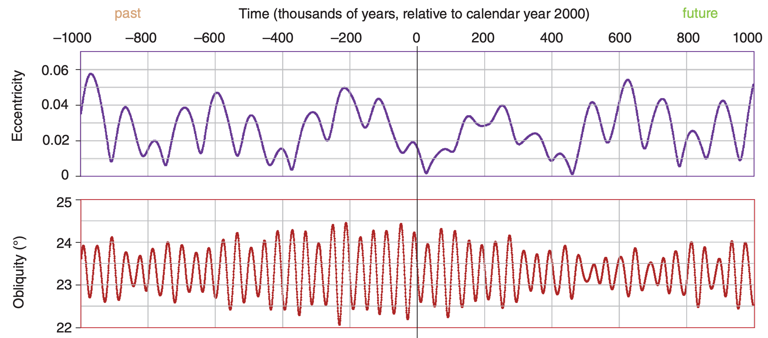
Fig. 21.8 shows eccentricity (purple curve at top) calculated using all 20 terms, for times ranging from 1 million years in the past to 1 million years into the future.
Sample Application
Plot ellipses for eccentricities of 0, 0.005, 0.058 & 0.50. Hints: the (x, y) coordinates are given by x = a·cos(t), and y = b·sin(t), where t varies from 0 to 2π radians. Assume a semi-major axis of a = 1, and get the semiminor axis from b = a·(1 – e2) 1/2.
Find the Answer
Plotted at right:
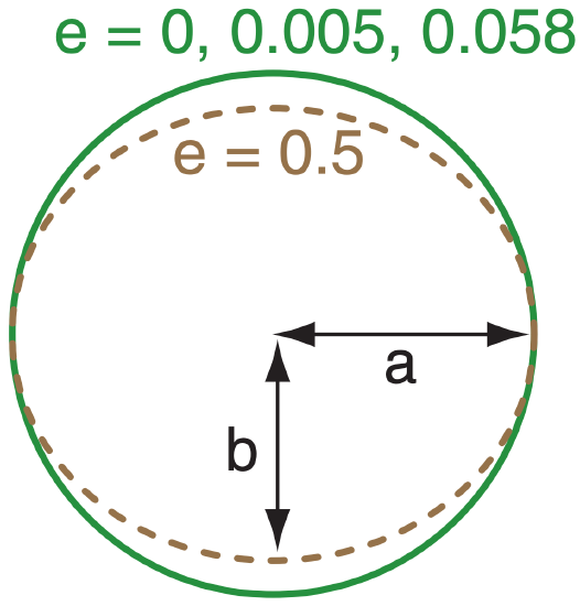
Exposition. The first 3 curves (solid green lines) look identical. Thus, for the full range of Earth’s eccentricities (0.0034 ≤ e ≤ 0.58), we see that Earth’s orbit is nearly circular (e = 0).
Sample Application.
Approximate the Earth-orbit eccentricity 600,000 years ago (i.e., 600,000 years before year 2000) using N = 5.
Find the Answer.
Given: t = –600,000 years (negative sign for past).
Find: e (dimensionless).
Use eq. (21.12) with data from Table 21-1: e ≈ 0.0275579
+ 0.010739·cos[2π·(–600000yr/405091yr + 170.739°/360°)]
+ 0.008147·cos[2π·(–600000yr/ 94932yr + 109.891°/360°)]
+ 0.006222·cos[2π·(–600000yr/123945yr – 60.044°/360°)]
+ 0.005287·cos[2π·(–600000yr/ 98857yr – 86.140°/360°)]
+ 0.004492·cos[2π·(–600000yr/130781yr + 100.224°/360°)]
e ≈ 0.0275579 + 0.0107290 + 0.0081106 + 0.0062148 – 0.0019045 – 0.0016384 ≈ 0.049 (dimensionless)
Check: 0.0034 ≤ e ≤ 0.058, within the expected eccentricity range for Earth. Almost agrees with the exact answer of 0.047 from Fig. 21.8, using all N = 20 terms.
Exposition: An interglacial (non-ice-age) period was ending, & a new glacial (ice-age) period was starting.
| Table 21-1. This table shows only the first 4 or 5 factors for the orbital series calculations, as used in the Sample Applications. To see all 20 to 26 factors, which were used to create Fig. 21.8, use Table 21-1b in section 21.10.3 near the end of this chapter. | |||
| index | A | P (years) | ϕ (degrees) |
| Eccentricity: | |||
|
i= 1 2 3 4 5 |
0.010739 0.008147 0.006222 0.005287 0.004492 |
405,091. 94,932. 123,945. 98,857. 130,781. |
170.739 109.891 –60.044 –86.140 100.224 |
| Obliquity: | |||
|
j= 1 2 3 4 |
0.582412° 0.242559° 0.163685° 0.164787° |
40,978. 39,616. 53,722. 40,285. |
86.645 120.859 –35.947 104.689 |
| Climatic Precession: | |||
|
k= 1 2 3 4 5 |
0.018986 0.016354 0.013055 0.008849 0.004248 |
23,682. 22,374. 18,953. 19,105. 23,123. |
44.374 –144.166 154.212 –42.250 90.742 |
| Simplified from Laskar, Robutel, Joutel, Gastineau, Correia & Levrard, 2004: A long-term numerical solution for the insolation quantities of the Earth. “Astronomy & Astrophysics”, 428, 261-285. | |||
By eye, we see two superimposed oscillations of eccentricity with periods of about 100 and 400 kyr (where “kyr” = kilo years = 1000 years). The first oscillation correlates very well with the roughly 100 kyr period for cool events associated with ice ages. The present eccentricity is about 0.0167. Short-term forecast: eccentricity will change little during the next 100,000 years. Variations in e affect Earth-sun distance R via eq. (2.4) in the Solar & IR Radiation chapter.
21.2.1.2. Obliquity
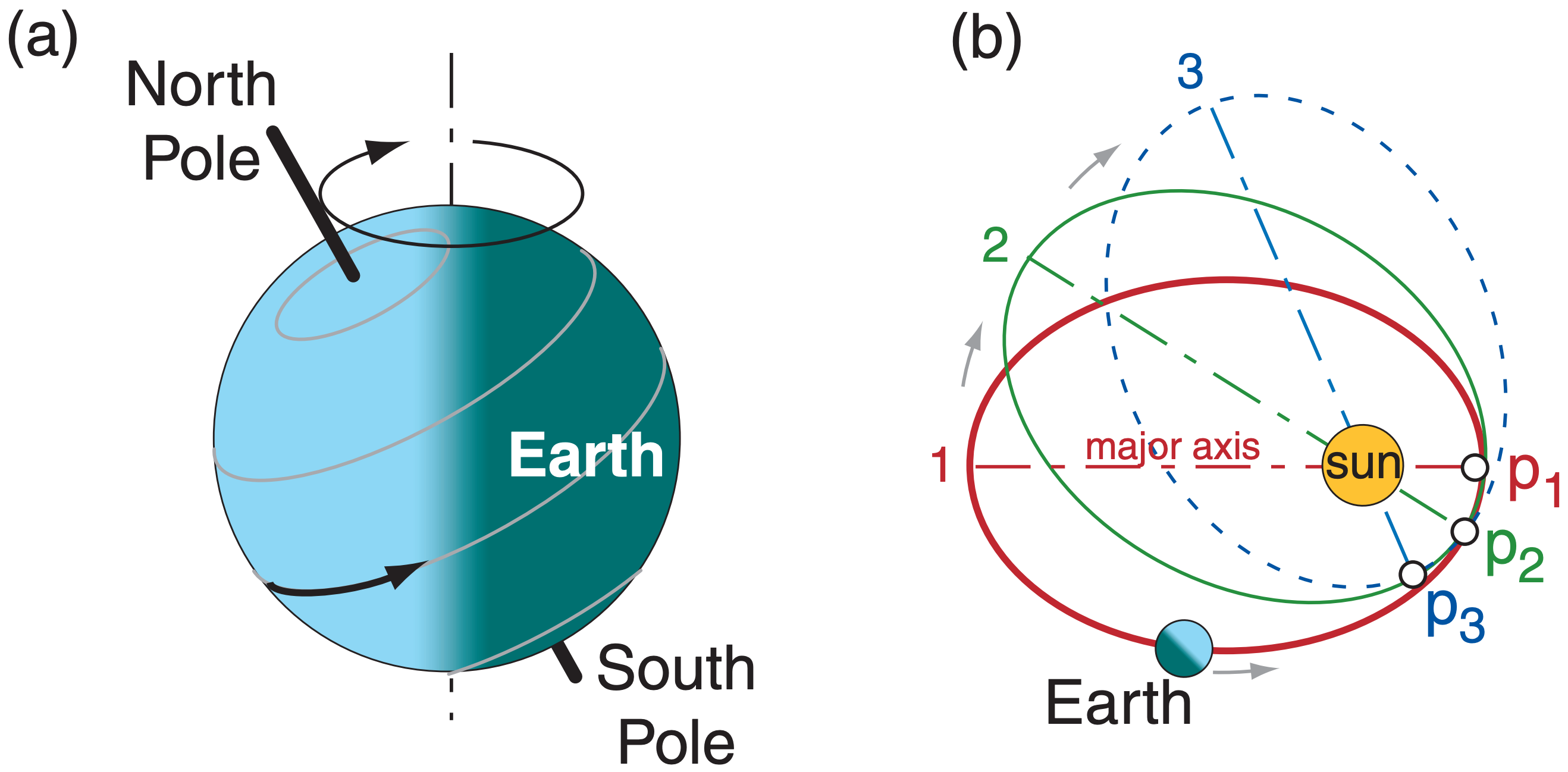
The tilt (obliquity) of Earth’s axis slowly fluctuates between 22.1° and 24.5°. This tilt angle is measured from a line perpendicular to Earth’s orbital plane (the ecliptic) around the sun (Fig. 21.7b).
A series approximation for obliquity ε is:
\begin{align}\varepsilon=\varepsilon_{o}+\sum_{j=1}^{N} A_{j} \cdot \cos \left[C \cdot\left(\frac{t}{P_{j}}+\frac{\phi_{j}}{360^{\circ}}\right)\right]\tag{21.13}\end{align}
where εo = 23.254500°, and all the other factors have the same meaning as for the eq. (21.12). Table 21-1 shows values for these orbital factors for N = 4 terms in this series, and Table 21-1b has all N = 23 terms.
The red curve in Fig. 21.8 shows that obliquity oscillates with a period of about 41,000 years. The present obliquity is 23.439° and is gradually decreasing.
Obliquity affects insolation via the solar declination angle (eq. 2.5 in the Solar & IR Radiation chapter, where a different symbol Φr was used for obliquity). Recall from the Solar & IR Radiation chapter that Earth-axis tilt is responsible for the seasons, so greater obliquity would cause greater contrast between winter and summer. One hypothesis is that ice ages are more likely during times of lesser obliquity, because summers would be cooler, causing less melting of glaciers.
21.2.1.3. Precession
Various precession processes affect climate.
Axial Precession. Not only does the tilt magnitude (obliquity) of Earth’s axis change with time, but so does the tilt direction. This tilt direction rotates in space, tracing one complete circle in 25,680 years (Fig. 21.9a) relative to the fixed stars. It rotates opposite to the direction the Earth spins. This precession is caused by the gravitational pull of the sun and moon on the Earth, because the Earth is an oblate spheroid (has larger diameter at the equator than at the poles). Hence, the Earth behaves somewhat like a spinning toy top.
Aphelion Precession. The direction of the major axis of Earth’s elliptical orbit also precesses slowly (with a 174,000 to 304,00 year period) relative to the fixed stars (Fig. 21.9b). The rotation direction is the same as the axial-precession, but the precession speed fluctuates due to the gravitational pull of the planets (mostly Jupiter and Saturn).
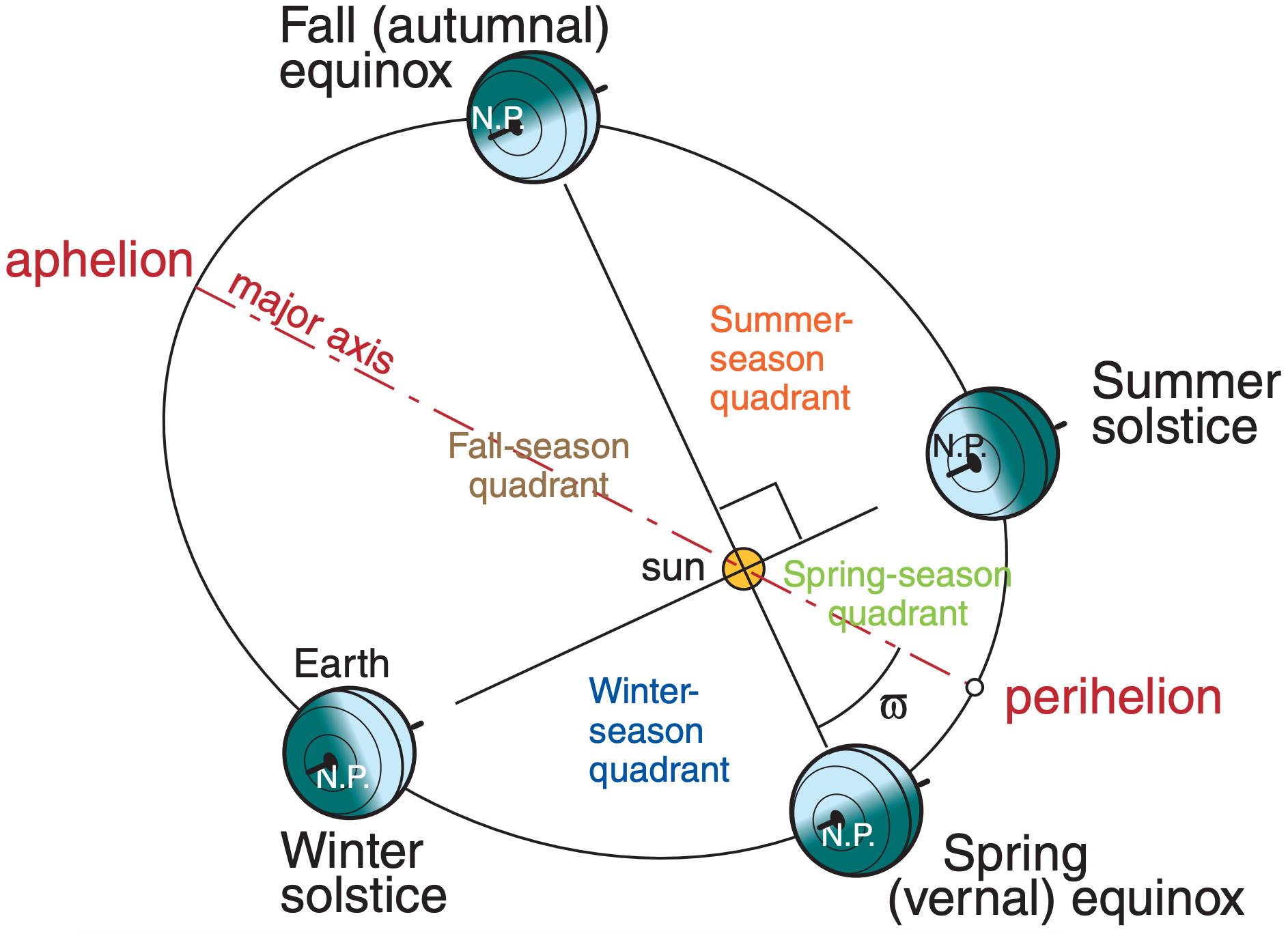
Equinox Precession. Summing axial and aphelion precession rates (i.e., adding the inverses of their periods) gives a total precession with fluctuating period of about 22,000 years. This combined precession describes changes to the angle (measured at the sun) between Earth’s orbital positions at the perihelion (point of closest approach) and at the moving vernal (Spring) equinox (Fig. 21.10). This fluctuating angle (ϖ, a math symbol called “variant pi”) is the equinox precession.
For years when angle ϖ is such that the winter solstice is near the perihelion (as it is in this century), then the cooling effect of the N. Hemisphere being tilted away from the sun is slightly moderated by the fact that the Earth is closest to the sun; hence winters and summers are not as extreme as they could be. Conversely, for years with different angle ϖ such that the summer solstice is near the perihelion, then the N. Hemisphere is tilted toward the sun at the same time that the Earth is closest to the sun — hence expect hotter summers and colder winters. However, seasons near the perihelion are shorter duration than seasons near the aphelion, which moderates the extremes for this latter case.
Climatic Precession. ϖ by itself is less important for insolation than the combination with eccentricity e: e·sin(ϖ) and e·cos(ϖ). These terms, known as the climatic precession, can be expressed by series approximations, where both terms use the same coefficients from Table 21-1b, for N = 26.
\begin{align}e \cdot \sin (\varpi) \approx \sum_{k=1}^{N} A_{k} \cdot \sin \left[C \cdot\left(\frac{t}{P_{k}}+\frac{\phi_{k}}{360^{\circ}}\right)\right]\tag{21.14}\end{align}
\begin{align}\left.e \cdot \cos (\varpi) \approx \sum_{k=1}^{N} A_{k} \cdot \cos \left[C \cdot\left(\frac{t}{P_{k}}+\frac{\phi_{k}}{360^{\circ}}\right)\right]\right]\tag{21.15}\end{align}
Other factors are similar to those in eq. (21.12).
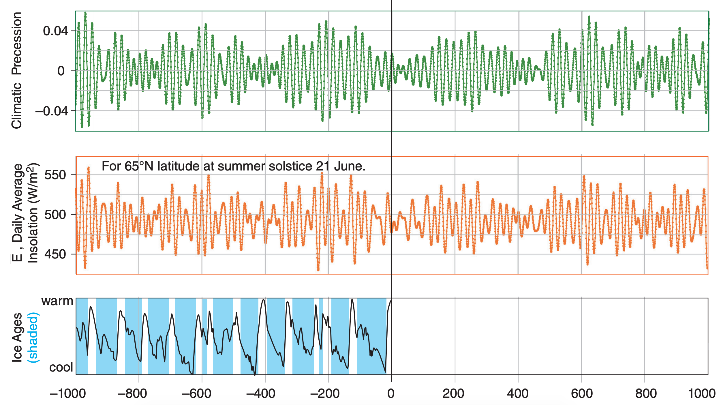
A plot of eq. (21.14), labeled “climatic precession”, is shown as the green curve in Fig. 21.8. It shows high frequency (22,000 year period) waves with amplitude modulated by the eccentricity curve from the top of Fig. 21.8. Climatic precession affects sunEarth distance, as described next.
Sample Application
Estimate the sine term of the climatic precession for year 2000, for N = 5.
Find the Answer
Given: t = 0
Find: e·sin(ϖ) = ? (dimensionless
Use eq. (21.14) with coefficients from Table 21-1.
e·sin(ϖ) =
+ 0.018986·[2π·(0yr/23682yr + 44.374°/360°)]
+ 0.016354·[2π·(0yr/22374yr – 144.166°/360°)]
+ 0.013055·[2π·(0yr/18953yr + 154.212°/360°)]
+ 0.008849·[2π·(0yr/19105yr – 42.250°/360°)]
+ 0.004248·[2π·(0yr/23123yr + 90.742°/360°)]
e·sin(ϖ) = 0.0132777 – 0.0095743 + 0.0056795
Check: This value is smaller than the exact value of 0.01628 from the curve plotted in Fig. 21.8.
Exposition: The eccentricity in year 2000 (i.e., almost at present) causes medium climatic precession.
| Table 21-2. Key values of λ, the angle between the Earth and the moving vernal equinox. Fig. 21.10 shows that solstices and equinoxes are exactly 90° apart. | |||
| Date | λ (radians, °) | sin(λ) | cos(λ) |
|---|---|---|---|
| Vernal (Spring) equinox | 0 , 0 | 0 | 1 |
| Summer solstice | π/2 , 90° | 1 | 0 |
| Autumnal (Fall) equinox | π , 180° | 0 | –1 |
| Winter solstice | 3π/2 , 270° | –1 | 0 |
21.2.1.4. Insolation Variations
Eq. (2.21) from the Solar & IR Radiation chapter gives average daily insolation \(\ \overline{E}\). It is repeated here:
\begin{align}\bar{E}=\frac{S_{O}}{\pi} \cdot\left(\frac{a}{R}\right)^{2} \cdot\left[h_{O}^{\prime} \cdot \sin (\phi) \cdot \sin \left(\delta_{S}\right)+\right.
\cos (\phi) \cdot \cos \left(\delta_{S}\right) \cdot \sin \left(h_{O}\right)\tag{21.16}\end{align}
where So =1361 W m–2 is the solar irradiance, a = 149.457 Gm is the semi-major axis length, R is the sun-Earth distance for any day of the year, ho’ is the hour angle in radians., ϕ is latitude, and δs is solar declination angle. Factors in this eq. are given next.
Instead of solving this formula for many latitudes, climatologists often focus on one key latitude: ϕ = 65°N. This latitude crosses Alaska, Canada, Greenland, Iceland, Scandinavia, and Siberia, and is representative of genesis zones for ice caps.
The hour angle ho at sunrise and sunset is given by the following set of equations:
\begin{align}\alpha=-\tan (\phi) \cdot \tan \left(\delta_{s}\right)\tag{21.17a}\end{align}
\begin{align}\beta=\min [1,(\max (-1, \alpha)]\tag{21.17b}\end{align}
\begin{align}h_{o}=\arccos (\beta)\tag{21.17c}\end{align}
Although the hour angle ho can be in radians or degrees (as suits your calculator or spreadsheet), the hour angle marked with the prime (ho’, in eq. 21.16) must be in radians.
The solar declination angle, used in eq. (21.16), is
\begin{align}\delta_{s}=\arcsin [\sin (\varepsilon) \cdot \sin (\lambda)] \approx \varepsilon \cdot \sin (\lambda)\tag{21.18}\end{align}
where ε is the obliquity from eq. (21.13), and λ is the true longitude angle (measured at the sun) between the position of the Earth and the position of the moving vernal equinox. Special cases for λ are listed in Table 21-2 on the previous page.
Recall from the Solar & IR Radiation chapter (eq. 2.4) that the sun-Earth distance R is related to the semi-major axis a by:
\begin{align}\frac{a}{R}=\frac{1+e \cdot \cos (v)}{1-e^{2}}\tag{21.19}\end{align}
where ν is the true anomaly (the angle at the sun between the Earth’s position and the perihelion), and e is the eccentricity. For the special case of the summer solstice (see the Sun-Earth Distance INFO Box), this becomes:
\begin{align}\frac{a}{R}=\frac{1+[e \cdot \sin (\varpi)]}{1-e^{2}}\tag{21.20}\end{align}
where e is from eq. (21.12) and e·sin(ϖ) is from eq. (21.14)
All the information above was used to solve eq. (21.16) for average daily insolation at latitude 65°N during the summer solstice for 1 Myr in the past to 1 Myr in the future. This results in the orange curve for \(\ \overline{ E}\) plotted in Fig. 21.8. This is the climatic signal resulting from Milankovitch theory. Some scientists have found a good correlation between it and the historical temperature curve plotted at the bottom of Fig. 21.8, although the issue is still being debated.
Sample Application
For the summer solstice at 65°N latitude, find the average daily insolation for years 2000 and 2200, using the small number of N values given in Table 21-1.
Find the Answer
Given: λ = π/2, ϕ = 65°N, (a) t = 0 , (b) t = 200 yr
Find: \(\ \overline{E}\) = ? W m–2 (Assume So = 1361 W m–2 = const.)
(a) From previous statements and Sample Applications: e = 0.0167, δs = ε = 23.439°, e·sin(ϖ) = 0.00768 Use eq. (21.17): ho = arccos[–tan(65°)·tan(23.439°)] = 158.4° = 2.7645 radians = ho’ .
Eq. (21.20): (a/R) = (1+0.00768)/[1–(0.0167)2] = 1.00796
Plugging all these into eq. (21.16):
\(\ \overline{E}\) = [(1361 W m–2)/π] ·(1.00796)2 · [2.7645 ·sin(65°) ·sin(23.439°) + cos(65°)·cos(23.439°)·sin(158.4°)]
\(\ \overline{E}\) = 501.48 W m–2 for t = 0.
(b) Eq. (21.12) for t = 200: e ≈ 0.0168
Eq. (21.13): ε = 23.2278°. Eq. (21.14): e·sin(ϖ) = 0.00730
Eq. (21.20): a/R = 1.00758. Eq. (21.16): \(\ \overline{E}\) = 497.5 W m–2
Check: Units OK. Magnitude ≈ that in Fig. 2.11 (Ch. 2) at the summer solstice (relative Julian day = 172).
Exposition: Milankovitch theory indicates that insolation will decrease slightly during the next 200 yr.
Recall from Chapter 2 (eq. 2.4) that the sun-Earth distance R is related to the semi-major axis a by:
\frac{a}{R}=\frac{1+e \cdot \cos (v)}{1-e^{2}}
\begin{align}\frac{a}{R}=\frac{1+e \cdot \cos (v)}{1-e^{2}}\tag{21.19}\end{align}
where ν is the true anomaly (angle at the sun between Earth’s position and the perihelion), and e is the eccentricity from eq. (21.12). By definition, νλϖ = − (21.a) where λ is the position of the Earth relative to the moving vernal equinox, and ϖ is the position of the perihelion as measured from the moving vernal equinox. Thus,
\begin{align}\frac{a}{R}=\frac{1+e \cdot \cos (\lambda-\varpi)}{1-e^{2}}\tag{21.b}\end{align}
Using trigonometric identities, the cosine term is:
\begin{align}\frac{a}{R}=\frac{1+\cos (\lambda) \cdot[e \cdot \cos (\varpi)]+\sin (\lambda) \cdot[e \cdot \sin (\varpi)]}{1-e^{2}}\tag{21.c}\end{align}
The terms in square brackets are the climatic precessions that you can find with eqs. (21.14) and (21.15).
To simplify the study of climate change, researchers often consider a special time of year; e.g., the summer solstice (λ = π/2 from Table 21-2). This time of year is important because it is when glaciers may or may not melt, depending on how warm the summer is. At the summer solstice, the previous equation simplifies to:
\begin{align}\frac{a}{R}=\frac{1+[e \cdot \sin (\varpi)]}{1-e^{2}}\tag{21.20}\end{align}
Also, during the summer solstice, the solar declination angle from eq. (21.18) simplifies to: δs = ε
21.2.2. Solar Output
The average total solar irradiance (TSI) currently reaching the top of Earth’s atmosphere is So = 1361 W·m–2, but the magnitude fluctuates daily due to solar activity, with extremes of 1358 and 1363 W·m–2 measured by satellite since 1975. Satellite observations have calibration errors (biases) on the order of ±4.5 W·m–2 (Kopp & Lean, 2011, Fig. 1).
21.2.2.1. Sunspot Cycle
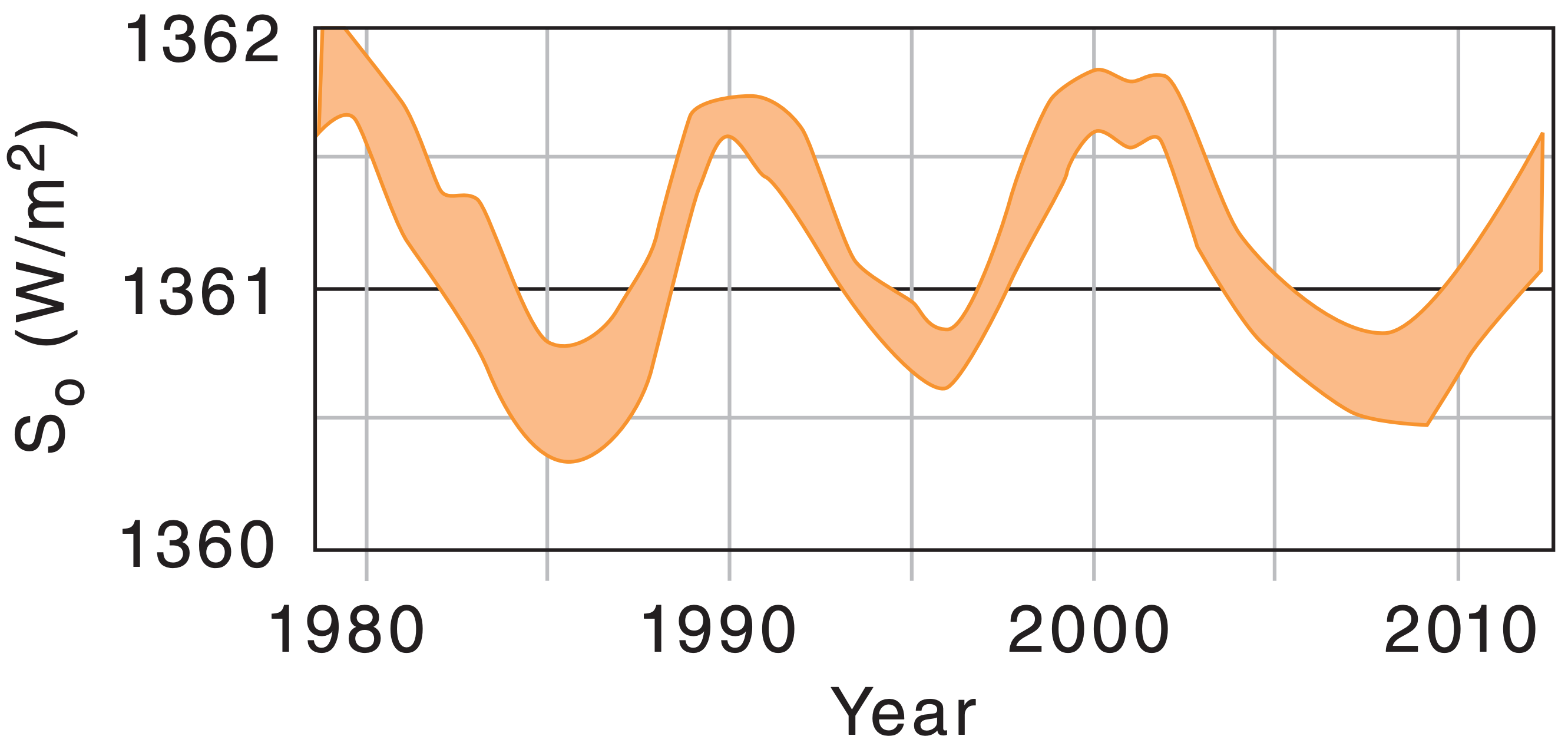
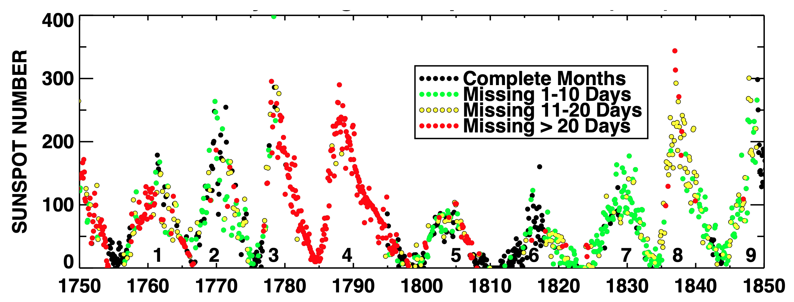
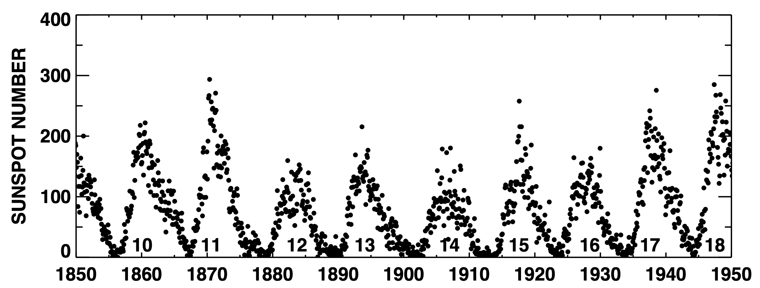
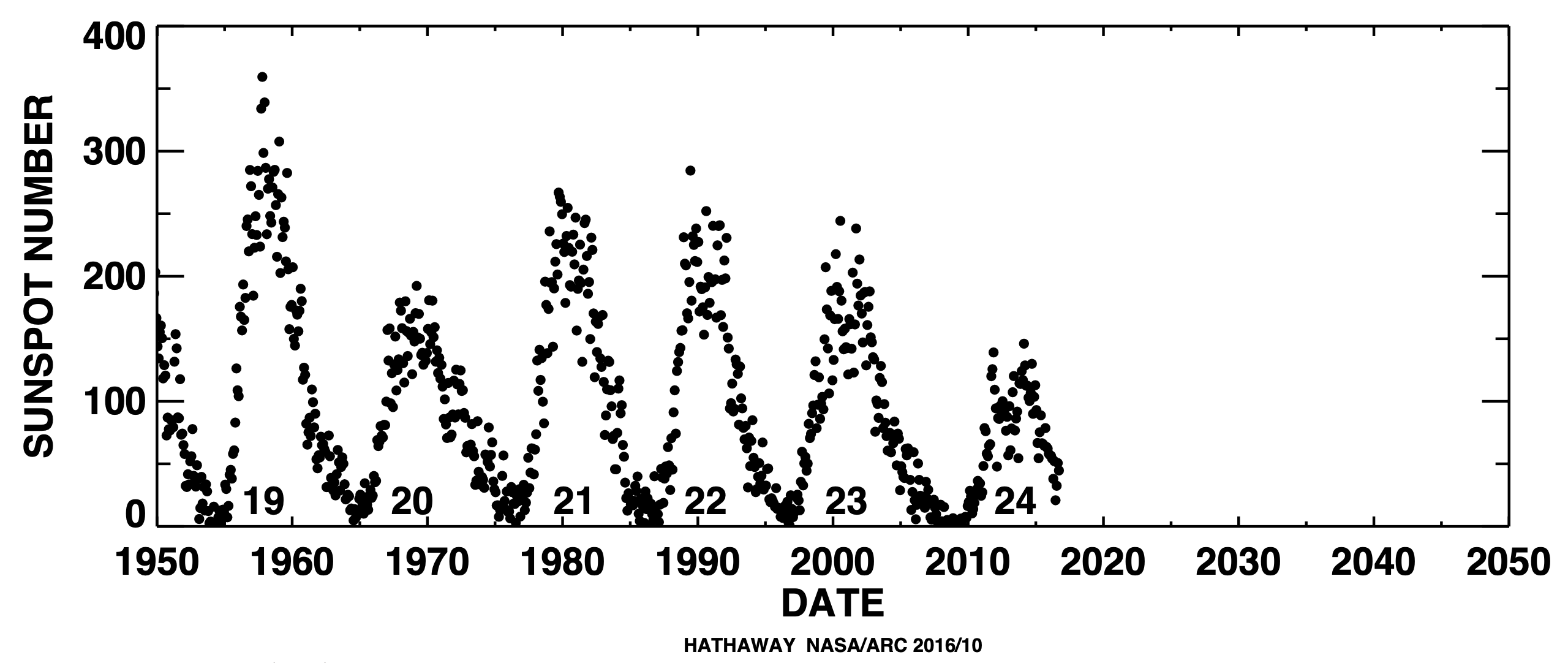
When averaged over each year, the resulting smoothed curve of TSI varies with a noticeable 11- yr cycle (Fig. 21.11), corresponding to the 9.5 to 11-yr sunspot cycle (Fig. 21.12) as observed by telescope.
Sunspots are darker and colder than the average surface temperature of the sun. However, sunspots are accompanied by faculae, which are brighter, hotter regions that often surround each sunspot. More sunspots means more faculae, and more faculae mean greater TSI.
Because the TSI variation is only about 0.1% of its total magnitude, the sunspot cycle is believed to have only a minor (possibly negligible) effect on recent climate change.
21.2.2.2. Long-term Variations in Solar Output
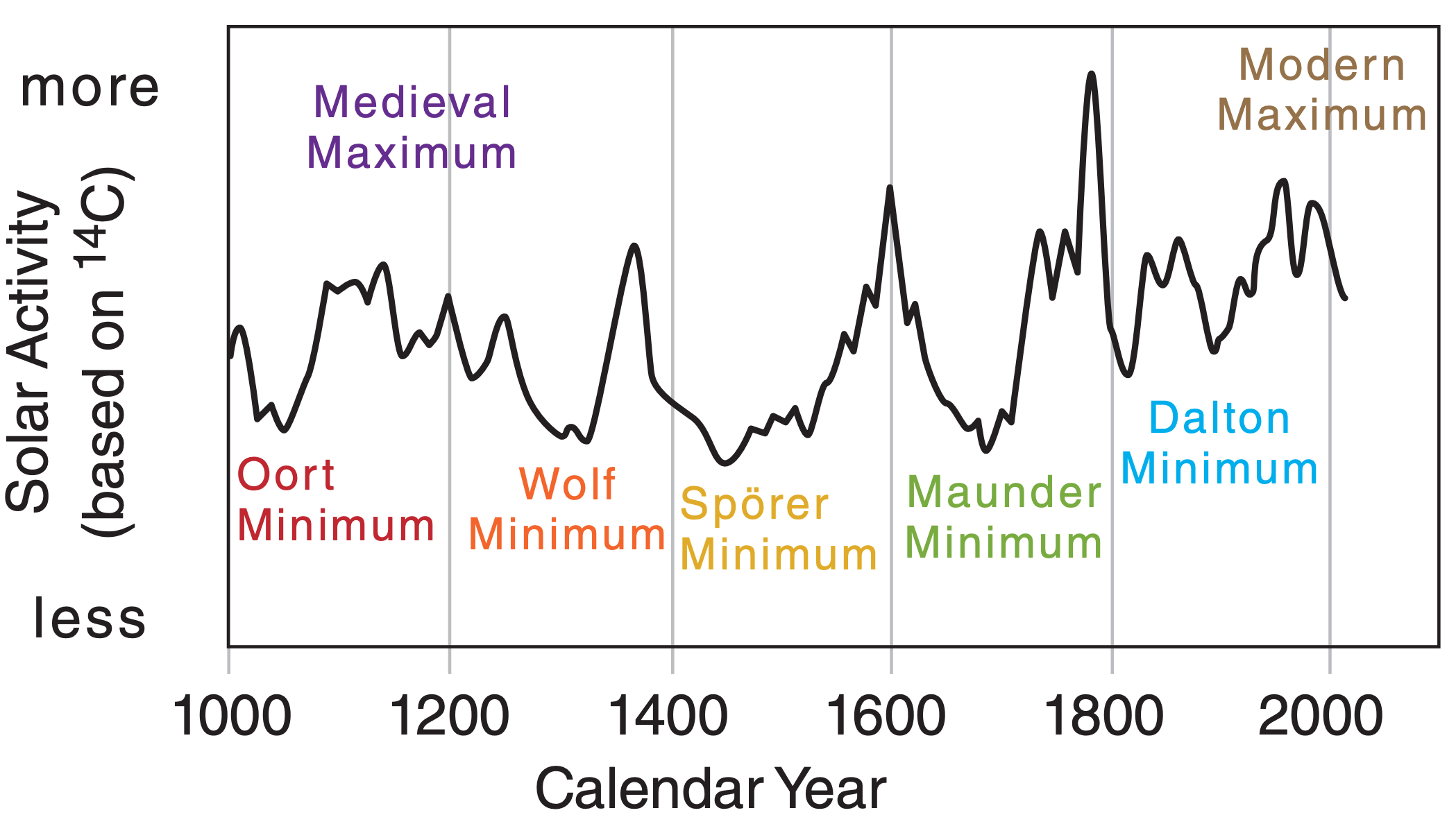
To get solar output information for the centuries before telescopes were invented, scientists use proxy measures. Proxies are measurable phenomena that vary with solar activity, such as beryllium-10 concentrations in Greenland ice cores, or carbon-14 concentration in tree rings (dendrochronology). Radioactive carbon-14 dating suggests solar activity as plotted in Fig. 21.13 for the past 1,000 years. Noticeable is the 200-yr cycle in solar-activity minima.
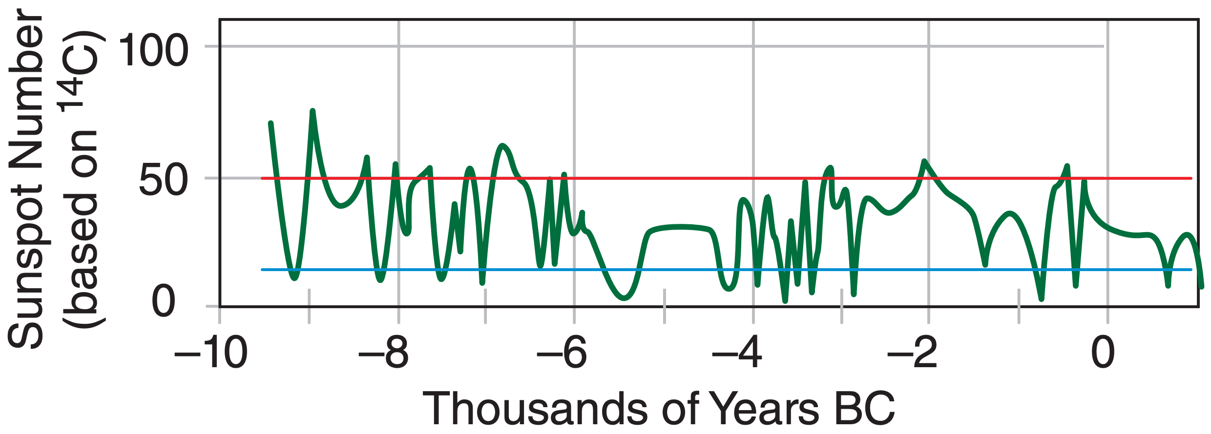
Going back 10,000 yr in time, Fig. 21.14 shows a highly-smoothed carbon-14 (14C) estimate of solar/ sunspot activity. There is some concern among scientists that Earth-based factors (such as extensive volcanic eruptions that darken the sky and reduce tree growth over many decades) may have confounded the proxy analysis of tree rings.
Even further back (4.5 Gyr ago), the sun was younger and weaker, and emitted only about 70% of what it currently emits. About 5 billion years into the future, the sun will grow into a red-giant star (killing all life on Earth), and later will shrink to become a white dwarf star.