21.1: Radiative Balance

Consider an Earth with no atmosphere (Fig. 21.1). Given the near-constant climate described above, assume a balance of radiation input and output.
Incoming solar radiation minus the portion reflected, multiplied by the area intercepted by Earth, gives the total radiative input:

\begin{align}\text {Radiation } \operatorname{In}=(1-A) \cdot S_{o} \cdot \pi \cdot R_{\text {Earth}}^{2}\tag{21.1}\end{align}

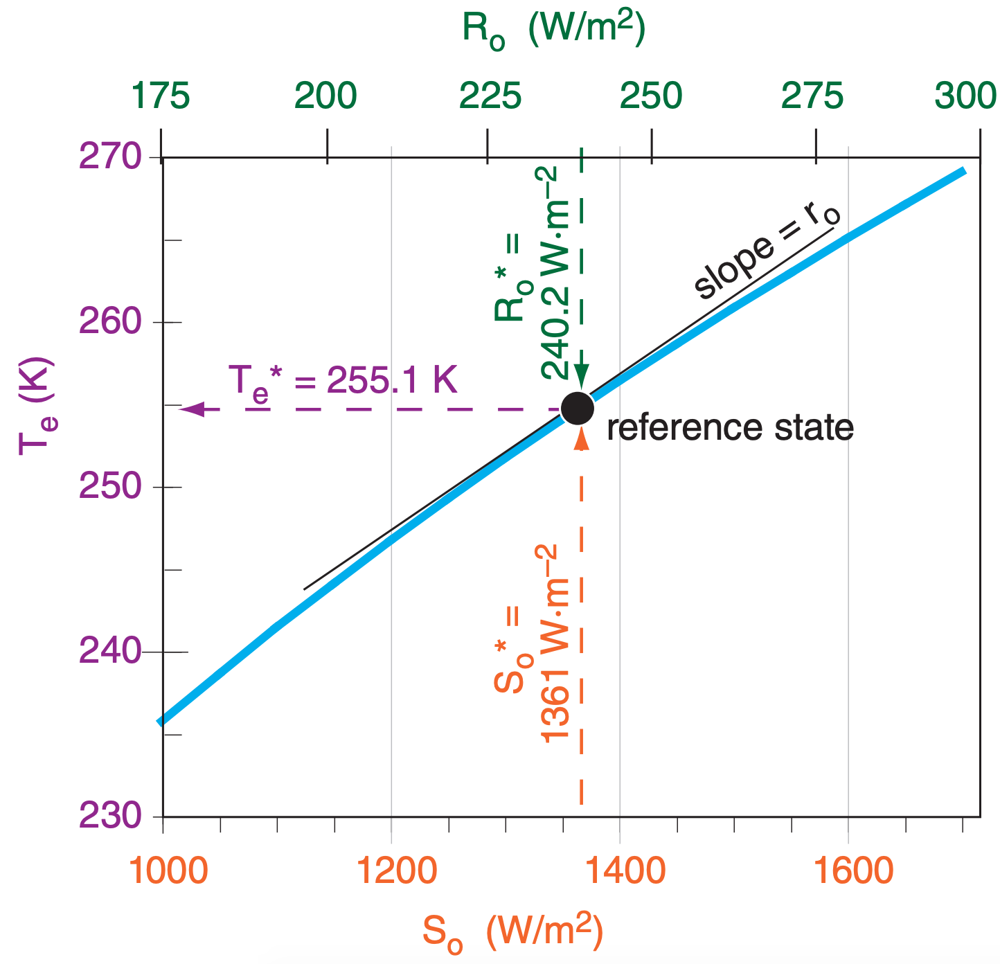
where the fraction reflected (A = 0.294) is called the global albedo (see INFO Box). The annual-average total solar irradiance (TSI) over all wavelengths as measured by satellites is S_o = 1361 W·m^–2. The interception area is the same as the area of Earth’s shadow — a disk of area πR_Earth², where R_Earth = 6371 km is the average radius of Earth. The TSI has fluctuated about ±0.5 W·m^–2 (the thickness of the vertical dashed line in Fig. 21.2) during the past 33 years due to the average sunspot cycle. See the Solar & IR Radiation chapter for TSI details.

Figure 21.1 Earth’s radiation balance of solar energy in and infrared (IR) radiation out.

Figure 21.2 Thick curved cyan line shows how the effective radiation temperature T_e for Earth varies with changes in solar irradiance S_o, given global albedo A = 0.294. Dashed lines show present conditions, which will be used as a reference point or reference state (R_o*, T_e*). Thin black straight line shows the slope r_o of the curve at the reference point. R_o = (1–A)·S_o/4 is net solar input for each square meter of the Earth’s surface (see INFO Box, next page).

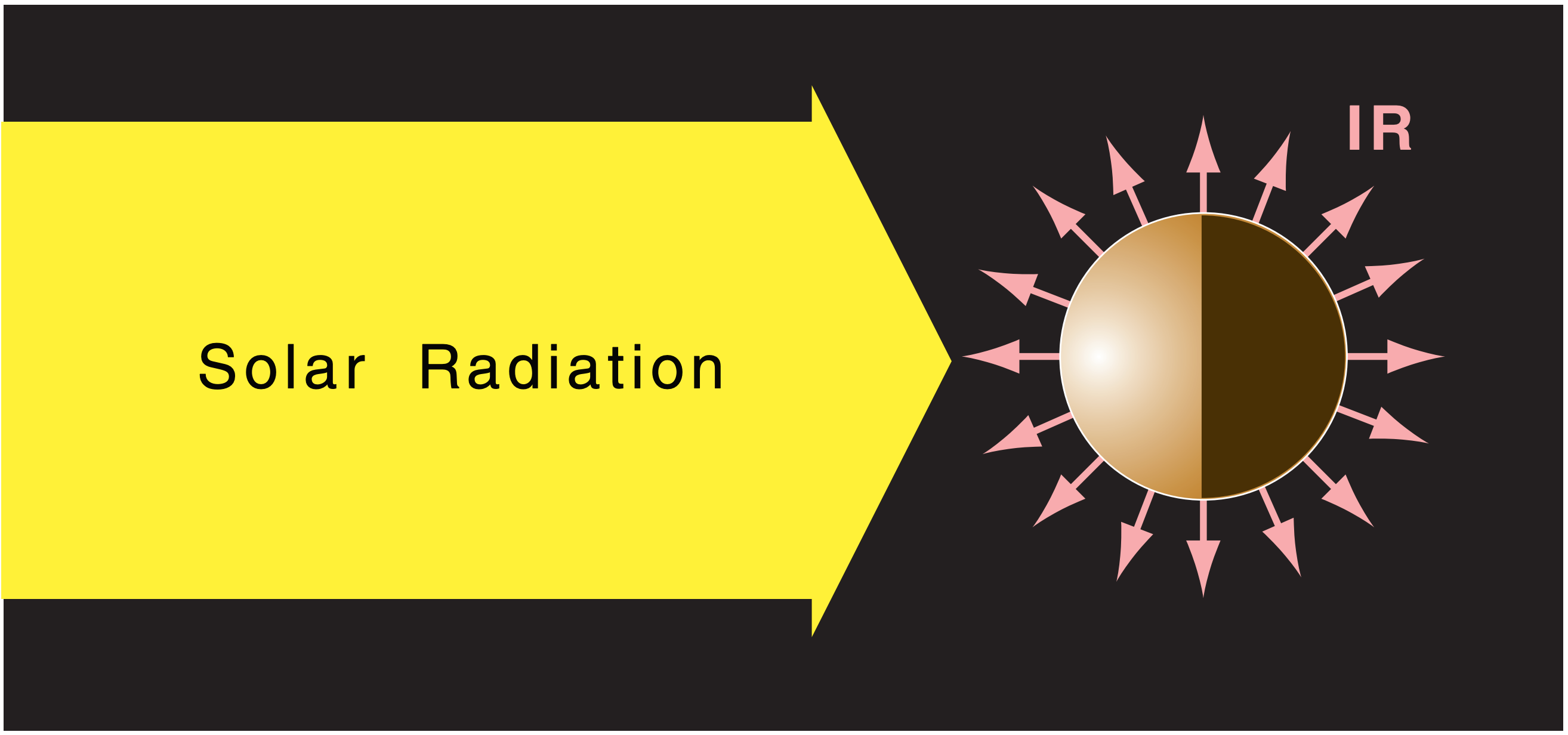
IR radiation is emitted from every point on Earth’s surface, which we will assume to behave as a radiative blackbody (emissivity = 1). For this toy model, assume that the earth is spherical with surface area 4·πR_Earth². If IR emissions/area are given by the Stefan-Boltzmann law (eq. 2.15), then the total outgoing radiation is:

\begin{align}\text {Radiation Out }=4 \pi \cdot R_{\text {Earth}}^{2} \cdot \sigma_{S B} \cdot T_{e}^{4}\tag{21.2}\end{align}

where the Stefan-Boltzmann constant is σ_SB = 5.67x10^–8 W·m^–2·K^–4.

The real Earth has a heterogeneous surface with cold polar ice caps, warm tropical continents, and other temperatures associated with different terrestrial and aquatic geographic features. Define an effective radiation emission temperature (T_e) such that the emissions from a hypothetical earth of uniform surface temperature T_e is the same as the total heterogeneous-Earth emissions.

For a steady-state climate (i.e., no temperature change with time), outputs must balance the inputs. Thus, equate outgoing and incoming radiation from eqs. (21.1 and 21.2), and then solve the resulting equation for T_e :

\begin{align}
T_{e} &=\left[\dfrac{(1-A) \cdot S_{o}}{4 \cdot \sigma_{S B}}\right]^{1 / 4}=\left[\dfrac{R_{o}}{\sigma_{S B}}\right]^{1 / 4}
\approx 255.1 \mathrm{K} \approx-18.0^{\circ} \mathrm{C}\tag{21.3}\end{align}

where R_o = (1–A)·S_o/4.

Fig. 21.2 shows this reference state at 255.1K, given an albedo of 0.294. It also shows how changes of solar irradiance along the abscissa of the graph need only small changes in effective temperature along the ordinate in order to reach a new radiative equilibrium. Namely, the radiation balance describes a negative feedback that causes a stable climate rather than runaway global warming.

Sample Application

Show the calculations leading to T_e = –18.0°C.

Given: T_e = –18.0°C, S_o = 1361 W·m^–2 , A = 0.294

Find: Show the calculation

Use eq. (21.3):

\(\ T_{e} =\left[\dfrac{(1-0.294) \cdot\left(1361 \mathrm{W} \cdot \mathrm{m}^{-2}\right)}{4 \cdot\left(5.67 \times 10^{-8} \mathrm{W} \cdot \mathrm{m}^{-2} \cdot \mathrm{K}^{-4}\right)}\right]^{1 / 4}
=255.1 \mathrm{K}=\bf{-18.0^{\circ} \mathrm{C}}\)

Check: Physics & units are OK.

Exposition: Earth’s radius appears in both the radiation-in and -out equations, but is not in eq. (21.3).

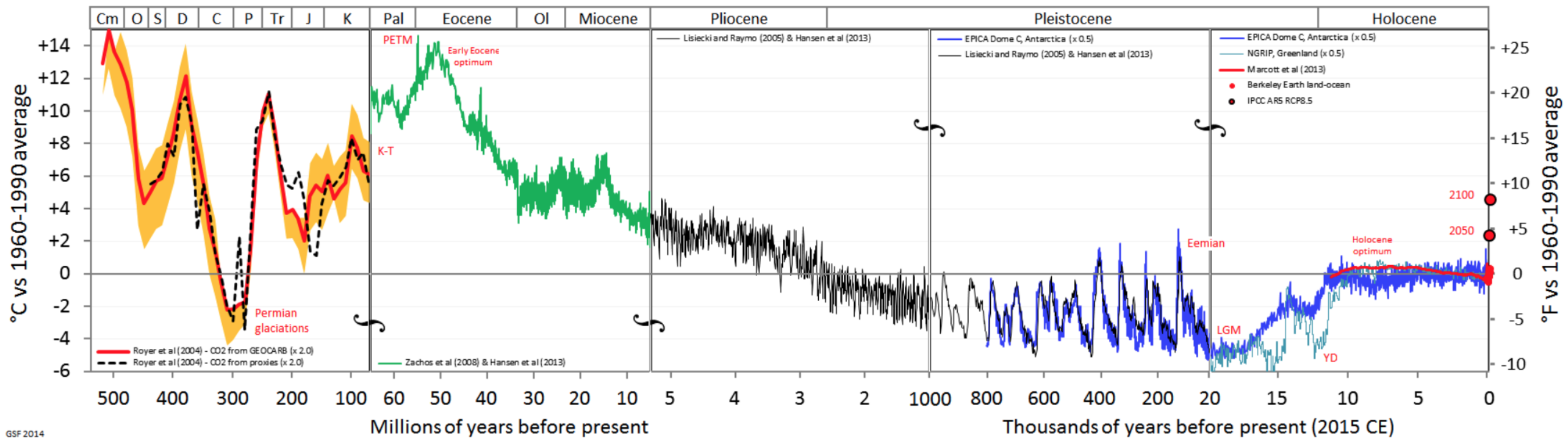
The geological record illustrates the steadiness of Earth’s past climate (Fig. 21.3). About 60 M years ago, the absolute temperature of Earth’s surface averaged roughly 5% warmer (i.e., 14 K = 14°C warmer ) than present. For the most recent 10 k years, the geologic record indicates temperature oscillations on the order of ±1°C relative to our current average surface temperature of 15°C. Nonetheless, these small temperature changes (with ∆T range of 20°C over the past 500 Myr) can cause significant changes in ice-cap coverage and sea level.

But our simple toy model is perhaps too simple, because the modeled –18.0°C temperature is colder than the +15°C actual surface temperature (from Chapter 1). To improve the modeled temperature, we must include some additional physics.

Figure 21.3 Paleotemperature estimate as a difference ∆T (°C) from the 1960 to 1990 temperature average. Scale breaks at the vertical lines. Note the ice-age cycles during 20 - 1000 k years ago. (By Glen Fergus - Own work, CC BY-SA 3.0, https://commons.wikimedia.org/w/index. php?curid=31736468 )

21.1.1. The So-called “Greenhouse Effect”

Figure 21.4 Simplified atmosphere-Earth system with greenhouse effect. Atmosphere thickness is exaggerated. R_o is the net solar input.

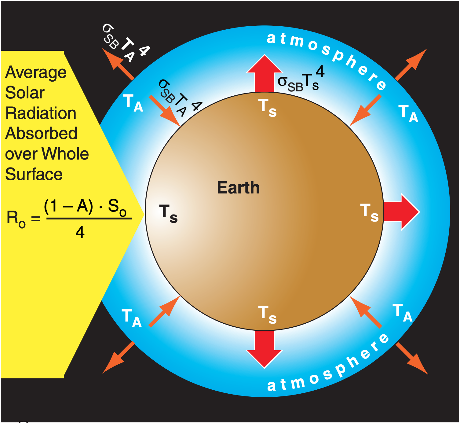
To make our Earth-system model slightly more realistic, add an atmosphere of uniform absolute temperature T_A everywhere (Fig 21.4). Suppose this atmosphere is opaque (not transparent) in the IR, but is perfectly transparent for visible light.

For this idealized case, sunlight shines through the atmosphere and reaches the Earth’s surface, where a portion is reflected and a portion is absorbed, causing the surface to warm. IR emitted from the warm Earth is totally absorbed by the atmosphere, causing the atmosphere to warm. But the atmosphere also emits radiation: some upward to space, and some back down to the Earth’s surface (a surface that absorbs 100% of the IR that hits it).

This downward IR from the atmosphere adds to the solar input, thus allowing the Earth’s surface to have a greater surface temperature T_s than with no atmosphere. This is called the greenhouse effect, even though real greenhouses do not work this way. Water vapor is one of many “greenhouse gases” that absorbs and emits IR radiation.

Assume the atmosphere-Earth system has existed for sufficient years to reach a steady state. Such an equilibrium state requires outgoing IR from the atmosphere-Earth system to balance absorbed incoming solar radiation. Namely:

\begin{align}T_{A}=T_{e}=255.1 \mathrm{K}=-18.0^{\circ} \mathrm{C}\tag{21.4}\end{align}

Thus, the temperature of the atmosphere must equal the effective emission temperature for the atmosphere-Earth system.

INFO • Why does R_o = (1–A)·S_o / 4 ?

In Figs. 21.4 and 21.5, the net solar input R_o is given as (1–A)·S_o/4 instead of S_o. The (1–A) factor is because any sunlight reflected back to space is not available to heat the Earth system. But why also divide by 4? The reason is due to geometry.

Of the radiation streaming outward from the sun, the shadow cast by the Earth indicates how much radiation was intercepted. The shadow is a circle with radius equal to the Earth’s radius R_Earth, hence the interception area is π·R_Earth².

But we prefer to study the energy fluxes relative to each square meter of the Earth’s surface. The surface area of a sphere is 4·π·R_Earth². Namely, the surface area is four times the area intercepted by the sun.

Hence, the average net solar input that we allocate to each square meter of the Earth’s surface is: R_o = (1–A)·S_o/4 = (1–0.294)·(1361 W·m–2)/4 = 240.2 W·m^–2.

You can use the Stefan-Boltzmann law σ_SB·T_A⁴ to find the radiation emitted both up and down from the atmosphere, which is assumed to be thin relative to Earth’s radius. For the atmosphere to be in steady-state, these two streams of outgoing IR radiation must balance the one stream of incoming IR from the Earth’s surface σ_SB·T_s⁴, which requires:

\begin{align}\sigma_{S B} \cdot T_{s}^{4}=2 \cdot \sigma_{S B} \cdot T_{e}^{4}\tag{21.5}\end{align}

Thus

\begin{align}
T_{s} &=2^{1 / 4} \cdot T_{e}
=303.4 \mathrm{K}=30.2^{\circ} \mathrm{C}\tag{21.6}\end{align}

While the no-atmosphere case was too cold, this opaque-atmosphere case is too warm (recall from Chapter 1 that the standard atmosphere T_s = 15°C). Perhaps the air is not fully opaque in the IR.

Sample Application

What temperature is the Earth’s surface for the one-layer atmosphere of the previous sample applic.

Find the Answer

Given: T_e = 255.1 K

Find: T_s = ? K

Apply eq. (21.6): T_s = 2^1/4·(255.1K) = 303.4 K = 30.2C

Check: Physics and units are OK.

Exposition: Twice the radiation at Earth’s surface, but not twice the surface absolute temperature.

21.1.2. Atmospheric Window

Figure 21.5 Idealized single-layer atmosphere having an IR dirty window.

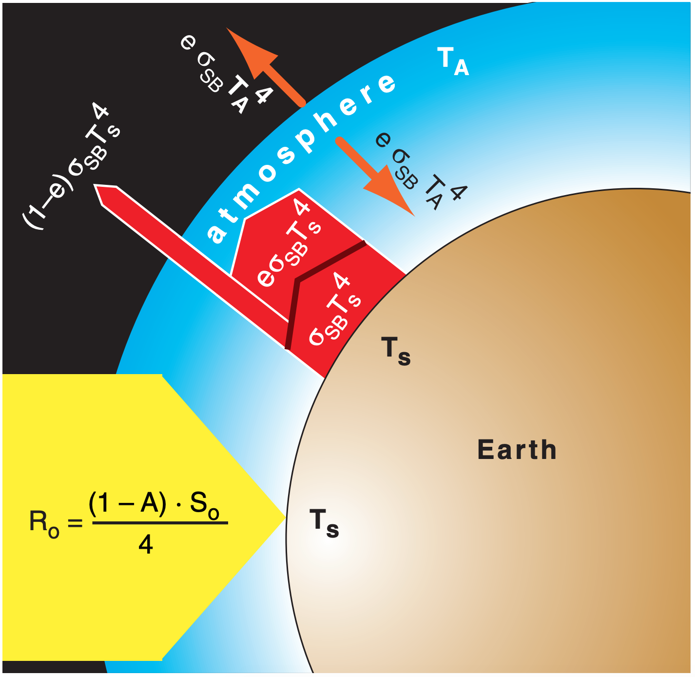
As discussed in the Satellites & Radar chapter, Earth’s atmosphere is partially transparent (i.e., is a dirty atmospheric window) for the 8 to 14 µm range of infrared radiation (IR) wavelengths and is mostly opaque at other wavelengths. Of all the IR emissions upward from Earth’s surface, suppose that 89.9% is absorbed and 10.1% escapes to space (Fig. 21.5). Thus, the atmosphere will not warm as much, and in turn, will not re-emit as much radiation back to the Earth’s surface.

At each layer (Earth’s surface, atmosphere, space) outgoing and incoming radiative fluxes balance for an Earth-system in equilibrium. Also, fluxes out of one layer are input to an adjacent layer. For example, the radiative balance of the atmosphere becomes

\begin{align}e_{\lambda} \cdot \sigma_{S B} \cdot T_{s}^{4}=2 \cdot e_{\lambda} \cdot \sigma_{S B} \cdot T_{A}^{4}\tag{21.7}\end{align}

while at the Earth’s surface it is

\begin{align}R_{o}+e_{\lambda} \cdot \sigma_{S B} \cdot T_{A}^{4}=\sigma_{S B} \cdot T_{s}^{4}\tag{21.8}\end{align}

From Kirchhoff’s law (see the Solar & IR Radiation chapter), recall that absorptivity equals emissivity, which for this idealized case is e_λ = a_λ = 89.9%. Eqs. (21.3, 21.7 & 21.8) can be combined to solve for key absolute temperatures:

\begin{align}T_{A}^{4}=\dfrac{T_{e}^{4}}{2-e_{\lambda}}\tag{21.9}\end{align}

\begin{align}T_{s}^{4}=\dfrac{2 \cdot T_{e}^{4}}{2-e_{\lambda}}\tag{21.10}\end{align}

where T_e is still given by eq. (21.4). The result is:

\(\ T_{A} \approx 249.1 \mathrm{K}=-24.1^{\circ} \mathrm{C}\)

and

\begin{align}T_{s} \approx 296.2 \mathrm{K}=23.0^{\circ} \mathrm{C}\tag{21.11}\end{align}

The temperature at Earth’s surface is more realistic, but is still slightly too warm.

A by-product of human industry and agriculture is the emission of gases such as methane (CH₄), carbon dioxide (CO₂), freon CFC-12 (C Cl₂ F₂), and nitrous oxide (N₂O) into the atmosphere. These gases, known as anthropogenic greenhouse gases, can absorb and re-emit IR radiation that would otherwise have been lost out the dirty window. The resulting increase of IR emissions from the atmosphere to Earth’s surface could cause global warming.

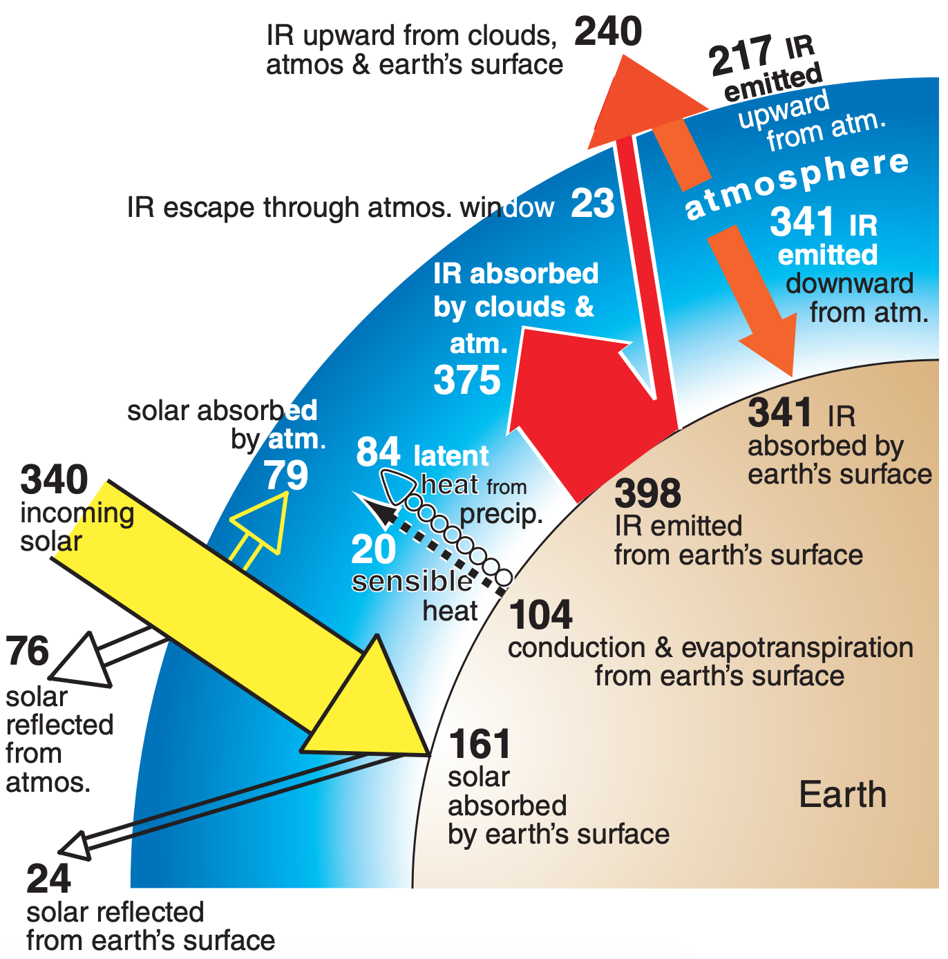
21.1.3. Average Energy Budget

Radiation is not the only physical process that transfers energy. Between the Earth and the bottom layer of the atmosphere there can be sensible-heat transfer via conduction (see the Thermodynamics chapter) and latent-heat transfer via evapotranspiration (see the Water Vapor chapter). Once this heat and moisture are in the air, they can be transported further into the atmosphere by the mean wind, by deep convection such as thunderstorms, by shallow convection such as thermals, and by smaller turbulent eddies in the atmospheric boundary layer.

One estimate of the annual mean of energy fluxes between all these components, when averaged over the surface area of the globe, is sketched in Fig. 21.6. According to the Stefan-Boltzmann law, the emitted IR radiation from the Earth’s surface (398 W·m^–2) corresponds to an blackbody surface temperature of 16.3°C, which is close to the observed value of 15°C.

Figure 21.6 Approximate global annual mean energy budget for the Earth system. The “atmosphere” component includes the air, clouds, and particles in the air. Numbers are energy fluxes in units of W·m^–2 relative to the Earth’s surface. Errors are of order 3% for fluxes at the top of the atmosphere, and errors are 5 to 25% for surface fluxes. The incoming solar radiation, when averaged over all the Earth’s surface, is S_o/4 = 340 W·m^–2. After subtracting the outgoing (reflected) solar radiation (340 – 76 – 24 = 240 W·m^–2), the result is the same R_o that we used before. [Based partially on IPCC AR5 Chapt. 2, Fig. 2.11, and Trenberth, Fasullo & Kiehl 2009, and Trenberth & Fasullo 2012. For sake of illustration, I modified the atmospheric IR emissions by 0.4% (within the reported noise range) to give a balanced budget. Instructors should encourage students to debate energy budget issues.]

Sample Application

Confirm that energy flows in Fig. 21.6 are balanced.

Find the Answer

Solar: incoming = [reflected] + (absorbed)

340 = [76 + 24] + (79 + 161)

340 = 340 W·m^–2

Earth’s surface: incoming = outgoing

(161 + 341) = (104 + 398)

502 = 502 W·m^–2

Atmosphere: incoming = outgoing

(79 + 20 + 84 + 375) = (217 + 341)

Earth System: in from space = out to space

340 = (24 + 76 + 23 + 217)

Check: Yes, all budgets are balanced.

Exposition: The solar budget must balance because the Earth-atmosphere system does not create/emit solar radiation. However, IR radiation is created by the sun, Earth, and atmosphere; hence, the IR fluxes by themselves need not balance.