13.6: Tendency of Sea-level Pressure
- Page ID
- 9615
\( \newcommand{\vecs}[1]{\overset { \scriptstyle \rightharpoonup} {\mathbf{#1}} } \)
\( \newcommand{\vecd}[1]{\overset{-\!-\!\rightharpoonup}{\vphantom{a}\smash {#1}}} \)
\( \newcommand{\id}{\mathrm{id}}\) \( \newcommand{\Span}{\mathrm{span}}\)
( \newcommand{\kernel}{\mathrm{null}\,}\) \( \newcommand{\range}{\mathrm{range}\,}\)
\( \newcommand{\RealPart}{\mathrm{Re}}\) \( \newcommand{\ImaginaryPart}{\mathrm{Im}}\)
\( \newcommand{\Argument}{\mathrm{Arg}}\) \( \newcommand{\norm}[1]{\| #1 \|}\)
\( \newcommand{\inner}[2]{\langle #1, #2 \rangle}\)
\( \newcommand{\Span}{\mathrm{span}}\)
\( \newcommand{\id}{\mathrm{id}}\)
\( \newcommand{\Span}{\mathrm{span}}\)
\( \newcommand{\kernel}{\mathrm{null}\,}\)
\( \newcommand{\range}{\mathrm{range}\,}\)
\( \newcommand{\RealPart}{\mathrm{Re}}\)
\( \newcommand{\ImaginaryPart}{\mathrm{Im}}\)
\( \newcommand{\Argument}{\mathrm{Arg}}\)
\( \newcommand{\norm}[1]{\| #1 \|}\)
\( \newcommand{\inner}[2]{\langle #1, #2 \rangle}\)
\( \newcommand{\Span}{\mathrm{span}}\) \( \newcommand{\AA}{\unicode[.8,0]{x212B}}\)
\( \newcommand{\vectorA}[1]{\vec{#1}} % arrow\)
\( \newcommand{\vectorAt}[1]{\vec{\text{#1}}} % arrow\)
\( \newcommand{\vectorB}[1]{\overset { \scriptstyle \rightharpoonup} {\mathbf{#1}} } \)
\( \newcommand{\vectorC}[1]{\textbf{#1}} \)
\( \newcommand{\vectorD}[1]{\overrightarrow{#1}} \)
\( \newcommand{\vectorDt}[1]{\overrightarrow{\text{#1}}} \)
\( \newcommand{\vectE}[1]{\overset{-\!-\!\rightharpoonup}{\vphantom{a}\smash{\mathbf {#1}}}} \)
\( \newcommand{\vecs}[1]{\overset { \scriptstyle \rightharpoonup} {\mathbf{#1}} } \)
\( \newcommand{\vecd}[1]{\overset{-\!-\!\rightharpoonup}{\vphantom{a}\smash {#1}}} \)
\(\newcommand{\avec}{\mathbf a}\) \(\newcommand{\bvec}{\mathbf b}\) \(\newcommand{\cvec}{\mathbf c}\) \(\newcommand{\dvec}{\mathbf d}\) \(\newcommand{\dtil}{\widetilde{\mathbf d}}\) \(\newcommand{\evec}{\mathbf e}\) \(\newcommand{\fvec}{\mathbf f}\) \(\newcommand{\nvec}{\mathbf n}\) \(\newcommand{\pvec}{\mathbf p}\) \(\newcommand{\qvec}{\mathbf q}\) \(\newcommand{\svec}{\mathbf s}\) \(\newcommand{\tvec}{\mathbf t}\) \(\newcommand{\uvec}{\mathbf u}\) \(\newcommand{\vvec}{\mathbf v}\) \(\newcommand{\wvec}{\mathbf w}\) \(\newcommand{\xvec}{\mathbf x}\) \(\newcommand{\yvec}{\mathbf y}\) \(\newcommand{\zvec}{\mathbf z}\) \(\newcommand{\rvec}{\mathbf r}\) \(\newcommand{\mvec}{\mathbf m}\) \(\newcommand{\zerovec}{\mathbf 0}\) \(\newcommand{\onevec}{\mathbf 1}\) \(\newcommand{\real}{\mathbb R}\) \(\newcommand{\twovec}[2]{\left[\begin{array}{r}#1 \\ #2 \end{array}\right]}\) \(\newcommand{\ctwovec}[2]{\left[\begin{array}{c}#1 \\ #2 \end{array}\right]}\) \(\newcommand{\threevec}[3]{\left[\begin{array}{r}#1 \\ #2 \\ #3 \end{array}\right]}\) \(\newcommand{\cthreevec}[3]{\left[\begin{array}{c}#1 \\ #2 \\ #3 \end{array}\right]}\) \(\newcommand{\fourvec}[4]{\left[\begin{array}{r}#1 \\ #2 \\ #3 \\ #4 \end{array}\right]}\) \(\newcommand{\cfourvec}[4]{\left[\begin{array}{c}#1 \\ #2 \\ #3 \\ #4 \end{array}\right]}\) \(\newcommand{\fivevec}[5]{\left[\begin{array}{r}#1 \\ #2 \\ #3 \\ #4 \\ #5 \\ \end{array}\right]}\) \(\newcommand{\cfivevec}[5]{\left[\begin{array}{c}#1 \\ #2 \\ #3 \\ #4 \\ #5 \\ \end{array}\right]}\) \(\newcommand{\mattwo}[4]{\left[\begin{array}{rr}#1 \amp #2 \\ #3 \amp #4 \\ \end{array}\right]}\) \(\newcommand{\laspan}[1]{\text{Span}\{#1\}}\) \(\newcommand{\bcal}{\cal B}\) \(\newcommand{\ccal}{\cal C}\) \(\newcommand{\scal}{\cal S}\) \(\newcommand{\wcal}{\cal W}\) \(\newcommand{\ecal}{\cal E}\) \(\newcommand{\coords}[2]{\left\{#1\right\}_{#2}}\) \(\newcommand{\gray}[1]{\color{gray}{#1}}\) \(\newcommand{\lgray}[1]{\color{lightgray}{#1}}\) \(\newcommand{\rank}{\operatorname{rank}}\) \(\newcommand{\row}{\text{Row}}\) \(\newcommand{\col}{\text{Col}}\) \(\renewcommand{\row}{\text{Row}}\) \(\newcommand{\nul}{\text{Nul}}\) \(\newcommand{\var}{\text{Var}}\) \(\newcommand{\corr}{\text{corr}}\) \(\newcommand{\len}[1]{\left|#1\right|}\) \(\newcommand{\bbar}{\overline{\bvec}}\) \(\newcommand{\bhat}{\widehat{\bvec}}\) \(\newcommand{\bperp}{\bvec^\perp}\) \(\newcommand{\xhat}{\widehat{\xvec}}\) \(\newcommand{\vhat}{\widehat{\vvec}}\) \(\newcommand{\uhat}{\widehat{\uvec}}\) \(\newcommand{\what}{\widehat{\wvec}}\) \(\newcommand{\Sighat}{\widehat{\Sigma}}\) \(\newcommand{\lt}{<}\) \(\newcommand{\gt}{>}\) \(\newcommand{\amp}{&}\) \(\definecolor{fillinmathshade}{gray}{0.9}\)Because cyclones are associated with low surface pressure, processes that lower the sea-level pressure (i.e., deepen the low) favor cyclogenesis. On isobaric surfaces such as 100 kPa, a deepening cyclone corresponds to falling geopotential heights.
Conversely, processes that cause rising sea-level pressure (i.e., filling the low) cause cyclolysis, or even anticyclogenesis. On an isobaric surface, this corresponds to rising geopotential heights.
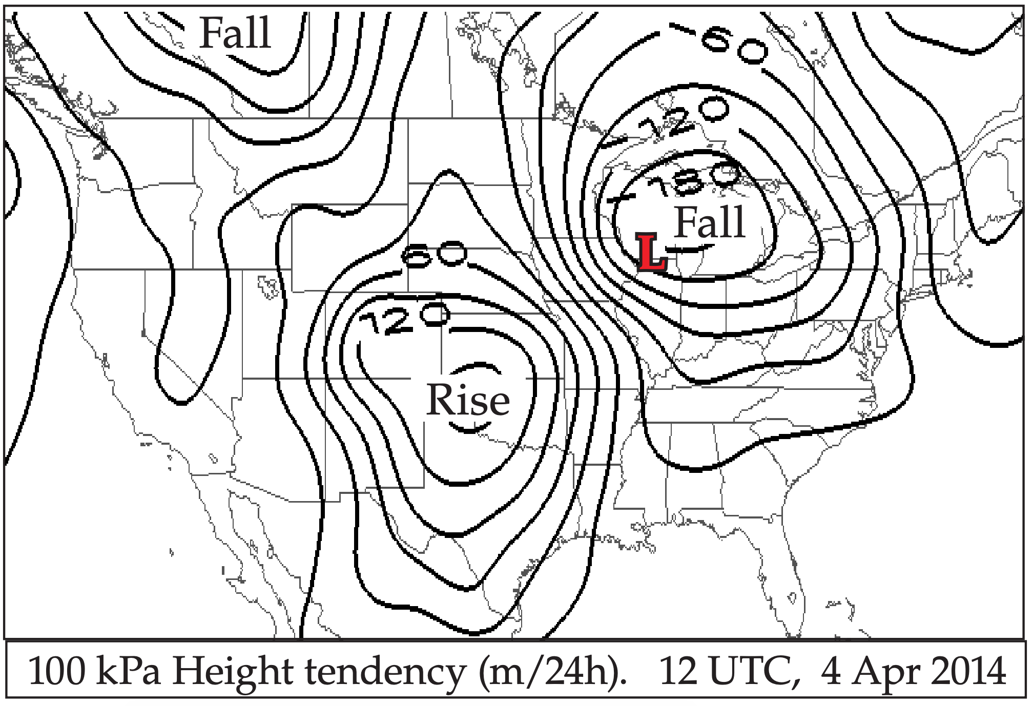
For an isobaric surface, the change of geopotential heights with time is called the height tendency (Fig. 13.42). The corresponding time variation of pressure on a constant height surface (e.g., sea-level) is known as pressure tendency. Given the close relationship between geopotential heights and pressures (recall Fig. 10.2 in the Atmospheric Forces and Winds chapter), falling heights correspond to falling pressures, both of which favor cyclogenesis.
13.6.1. Mass Budget
Because sea-level pressure depends on the weight of all the air molecules above it, a falling surface pressure must correspond to a removal of air molecules from the air column above the surface. An accounting of the total number of molecules in an air column is called a mass budget.
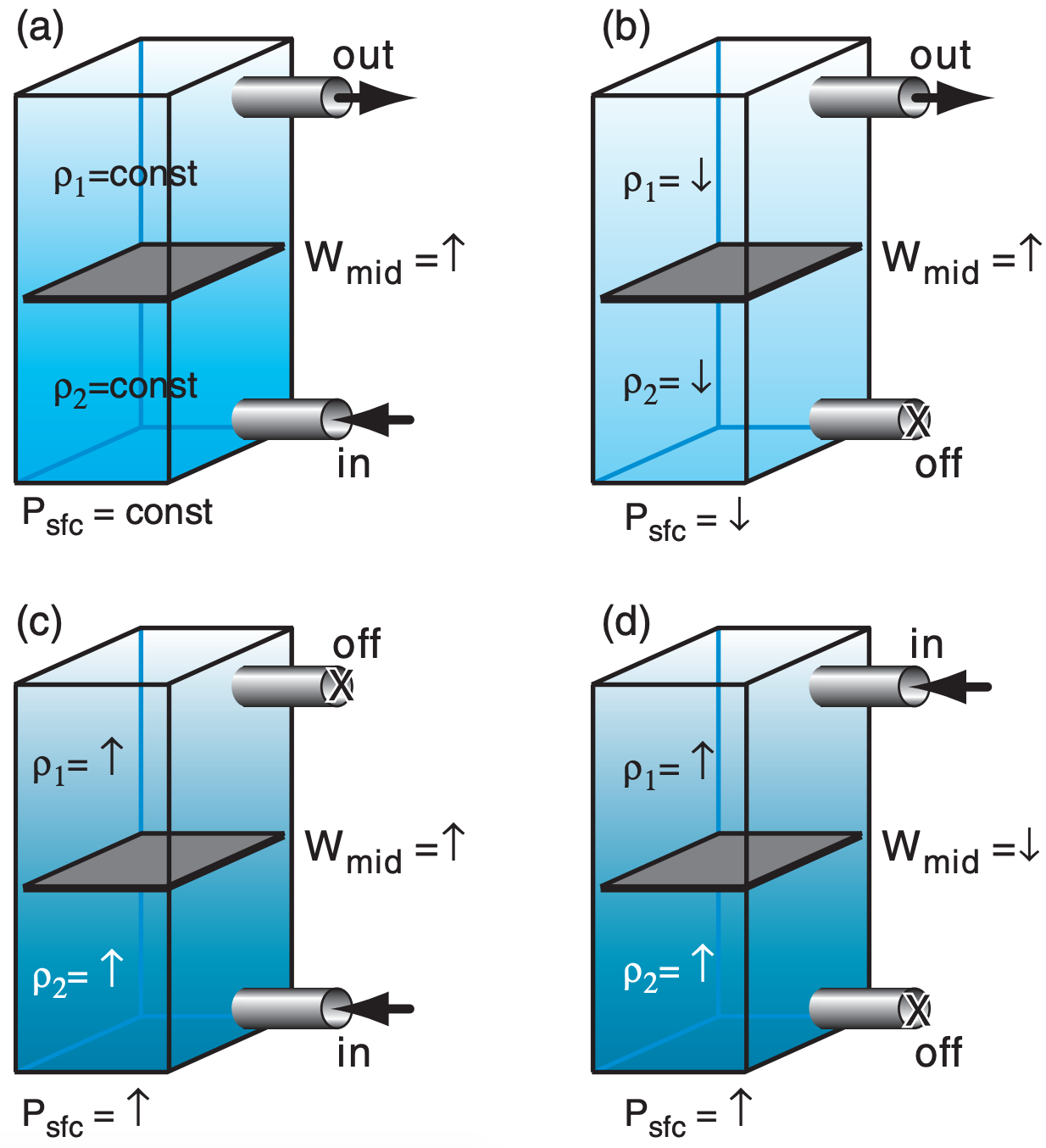
Imagine a column of air over 1 m2 of the Earth’s surface, as sketched in Fig. 13.43a. Suppose there is a weightless leaf (grey rectangle in that figure) that can move up and down with the air velocity Wmid in response to movement of air molecules in the column. Pick two arbitrary heights above and below the leaf, and consider the air densities at these heights. Because air is compressible, the density (ρ2) below the leaf is greater than the density (ρ1) above the leaf. But we will focus on how the densities at these fixed altitudes change for the scenarios below.
Scenario of Fig. 13.43a: Air is pumped into the bottom half of the column, while an equal amount of air molecules are pumped out of the top. Since mass_out = mass_in, the total mass in the column is constant. Therefore the surface pressure (Psfc) is constant, and the two densities do not change. But the leaf is pushed upward (Wmid = up) following the flow of air molecules upward in the column.
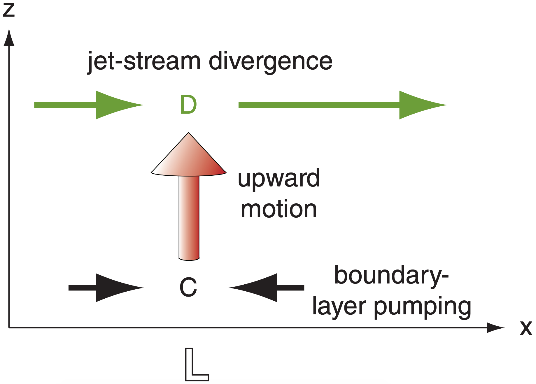
What could cause analogous inflows and outflows in the real atmosphere? Answers include: horizontal convergence of wind just above the surface, and divergence aloft in the jet stream.
Scenario of Fig 13.43b: Horizontal divergence of air aloft removes air molecules from the top of the air column, with no flow in or out of the bottom. As air molecules are evacuated from the column, the leaf moves upward, densities decrease, and surface pressure decreases because the fewer air molecules in the column cause less weight.
Scenario of Fig. 13.43c: Low-level convergence causes inflow, with no flow in or out of the top. As more molecules are pumped into the column, densities and surface pressure increase, and the leaf is pushed upward.
Scenario of Fig 13.43d: Horizontal convergence aloft causes inflow at the top of the column, with no flow in or out of the bottom. As more molecules enter the column, densities and surface pressure increase, but the leaf is pushed downward.
Pressure at sea level (Ps) is related to total column air mass (m) by:
\(\ \begin{align} P_{s}=\frac{|g|}{A} \cdot m\tag{13.34}\end{align}\)
where the column bottom surface has area (A) and gravitational acceleration is |g| = 9.8 m·s–2. If the column mass changes with time, then so must the surface pressure:
\(\ \begin{align} \frac{\Delta P_{S}}{\Delta t}=\frac{|g|}{A} \cdot \frac{\Delta m}{\Delta t}\tag{13.35}\end{align}\)
Suppose that a hypothetical column of height z contains constant-density air. You can relate density to mass by
\(\ \begin{align} m=\rho \cdot V o l u m e=\rho \cdot A \cdot z\tag{13.36}\end{align}\)
Thus, ∆m/∆t causes ∆z/∆t, where ∆z/∆t is vertical velocity Wsurrogate. Plugging the previous two equations into eq. (13.34) gives a way to estimate the tendency of surface pressure as a function of the motion of our hypothetical leaf Wsurrogate:
\(\ \begin{align} \frac{\Delta P_{s}}{\Delta t}=\pm|g| \cdot \rho(z) \cdot W_{\text {surrogate }}(z)\tag{13.37}\end{align}\)
assuming we know the density ρ(z) of the inflow or outflow air occurring at height z. Use the negative sign in eq. (13.37) if it is driven at the top of the troposphere, and positive sign if driven at the bottom.
Consider the following four processes that can cause inflow or outflow to/from the column:
- Advection
- Boundary-layer pumping
- Upper-level divergence
- Diabatic heating
We can estimate a Wsurrogate for the last three processes, and then add all the processes to estimate the net pressure tendency.
Sample Application
If the surface pressure is 100 kPa, how much air mass is in the whole air column above a 1 meter squared surface area?
Find the Answer
Given: A = 1 m2, Ps = 100 kPa
Find: m = ? kg
Rearrange eq. (13.34) to solve for m:
m = Ps·A/|g| = [(100 kPa)·(1 m2) ] / (9.8 m s–2)
But from Appendix A: 1 Pa = 1 kg·m–1·s–2 , thus: m = [(105 kg·m–1·s–2)·(1 m2) ] / (9.8 m s–2) = 10.2 x 10³ kg = 10.2 Mg
Check: Physics and units are reasonable.
Exposition: This calculation assumed that gravitational acceleration is approximately constant over the depth of the atmosphere.
Eq. 13.34 can be used for the pressure at any height in the atmosphere, but only if m represents the mass of air above that height. For example, if the tropopause is at pressure 25 kPa, then the mass of air above the tropopause is one quarter of the previous answer; namely, 2.55 Mg over each square meter.
Subtracting this value from the previous answer shows that of the total 10.2 Mg of mass in the atmosphere above a square meter, most of the air (7.65 Mg) is within the troposphere.
Advection moves a low-pressure region from one location to another. If you know the wind direction and speed Mc that is blowing the low-pressure air column toward you, and if you know (∆Ps / ∆s) how surface pressure changes with distance s between your location and the advecting column, then you can estimate the pressure tendency due to advection by ∆Ps /∆t|advection = –Mc·(∆Ps /∆s).
Recall from the Atmospheric Forces and Winds chapter that frictional drag in the boundary layer causes the horizontal wind to spiral inward toward a low-pressure center. Mass continuity requires that this horizontal inflow be balanced by vertical outflow WBL out of the top of the boundary layer. This boundary-layer pumping vertical velocity can be used with air density ρBL at the boundary-layer top in the pressure tendency equation:
∆Ps /∆t|B.L.Pumping = –|g|· ρBL · WBL .
\(\Delta P_{s} /\left.\Delta t\right|_{B . L . \text {Pumping}}=-|g| \cdot \rho_{B L} \cdot W_{B L}\)
Earlier in this chapter we saw how jet-stream curvature and jet-streak processes can cause upperlevel divergence (U.L.Diverg.), which can remove mass from an air column and cause cyclogenesis. The Wmid from that section, along with the average mid-level air density ρmid, can be used to give:
\(\Delta P_{s} /\left.\Delta t\right|_{U . L . \text { Diverg. }}=-|g| \cdot \rho_{m i d} \cdot W_{m i d}\)
Non-adiabatic heating (diabatic heating) can be caused by solar or IR radiation, by condensation of water vapor, and other factors. The effect of latent heating on the surface pressure is described next.
Sample Application
Divergence of air at the top of the troposphere removes air molecules from the top of a tropospheric column, causing a 0.1 m s–1 updraft at height 8 km above ground level (AGL). No other processes add or remove air mass. What is the corresponding surface pressure tendency?
Find the Answer
Given: z = 8 km, Wsurrogate(8 km) = 0.1 m s–1
Find: ∆Ps /∆t = ? kPa s–1
For air density at z = 8 km, assume a standard atmosphere. Use ρ = 0.5252 kg m–3.
Use eq. (13.37) with negative sign because the forcing is at the top of the troposphere:
∆Ps /∆t = – (9.8 m s–2)·(0.5252 kg m–3)·(0.01 m s–1)
= – 0.0515 kg·m–1·s–3 = –0.0515 Pa s–1
= – 5.15x10⁻⁵ kPa s–1
Check: Physics and units are reasonable.
Exposition: The corresponding hourly pressure tendency is ∆Ps /∆t = –0.185 kPa h–1. If this rapid deepening of the cyclone were to continue for 24 h, we would classify this explosive cyclogenesis as a cyclone bomb.
13.6.2. Latent Heating
Water vapor might condense into drops or deposit into ice crystals at some heights within an air column — releasing latent heat and warming the column. If some of these precipitation particles evaporate before reaching the ground, then they absorb latent heat and cool the column.
The precipitation that does reach the ground is related to the net amount of condensational heating during time interval ∆t by
\( \begin{align} \frac{\Delta T_{v}}{\Delta t}=\frac{a}{\Delta z} \cdot \frac{L_{v}}{C_{p}} \cdot \frac{\rho_{l i q}}{\rho_{a i r}} \cdot R R\tag{13.38}\end{align}\)
where RR is rainfall rate (mm h–1), Tv is average aircolumn virtual temperature, a = 10–6 km mm–1, ∆z is depth of the air column (km), the ratio of latent heat of vaporization to specific heat of air is Lv/Cp = 2500 K·kgair /kgliq, and where (ρair , ρliq ) are air and liquid-water densities, respectively, with ρliq = 1000 kg m–3).
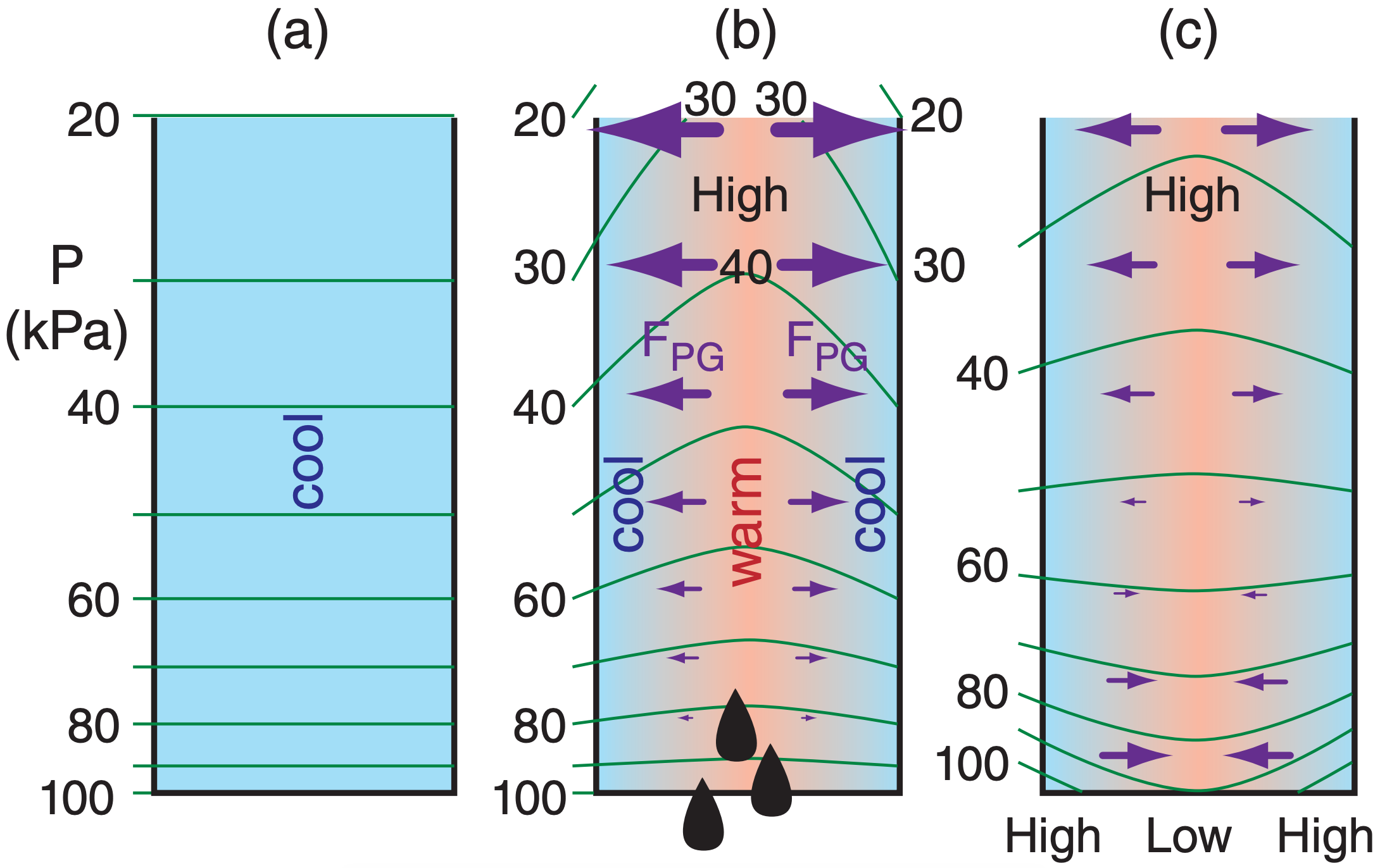
But the hypsometric equation relates pressure changes to temperature changes (Fig. 13.44). Thus, eq. (13.38) and the hypsometric equation can be merged to give:
\( \begin{align} \frac{\Delta P_{s}}{\Delta t}=-\frac{|g|}{\bar{T}_{v}} \cdot \frac{L_{v}}{C_{p}} \cdot \rho_{l i q} \cdot R R\tag{13.39}\end{align}\)
for an air column with average virtual temperature (Kelvin) of \(\ \overline{T_v}\) (≈ 300 K), and where gravitational acceleration magnitude is |g| = 9.8 m·s–2. Although latent heating and cooling might occur at different heights within the air column, eq. (13.39) describes the net column-average effect.
For a typical value of \(\ \overline{T_v}\), eq. (13.39) reduces to:
\(\ \begin{align} \frac{\Delta P_{S}}{\Delta t} \approx-b \cdot R R\tag{13.40}\end{align}\)
with factor \(b=\frac{|g|}{\bar{T}_{v}} \cdot \frac{L_{v}}{C_{p}} \cdot \rho_{l i q}\) ≈ 0.082 kPa mmrain–1
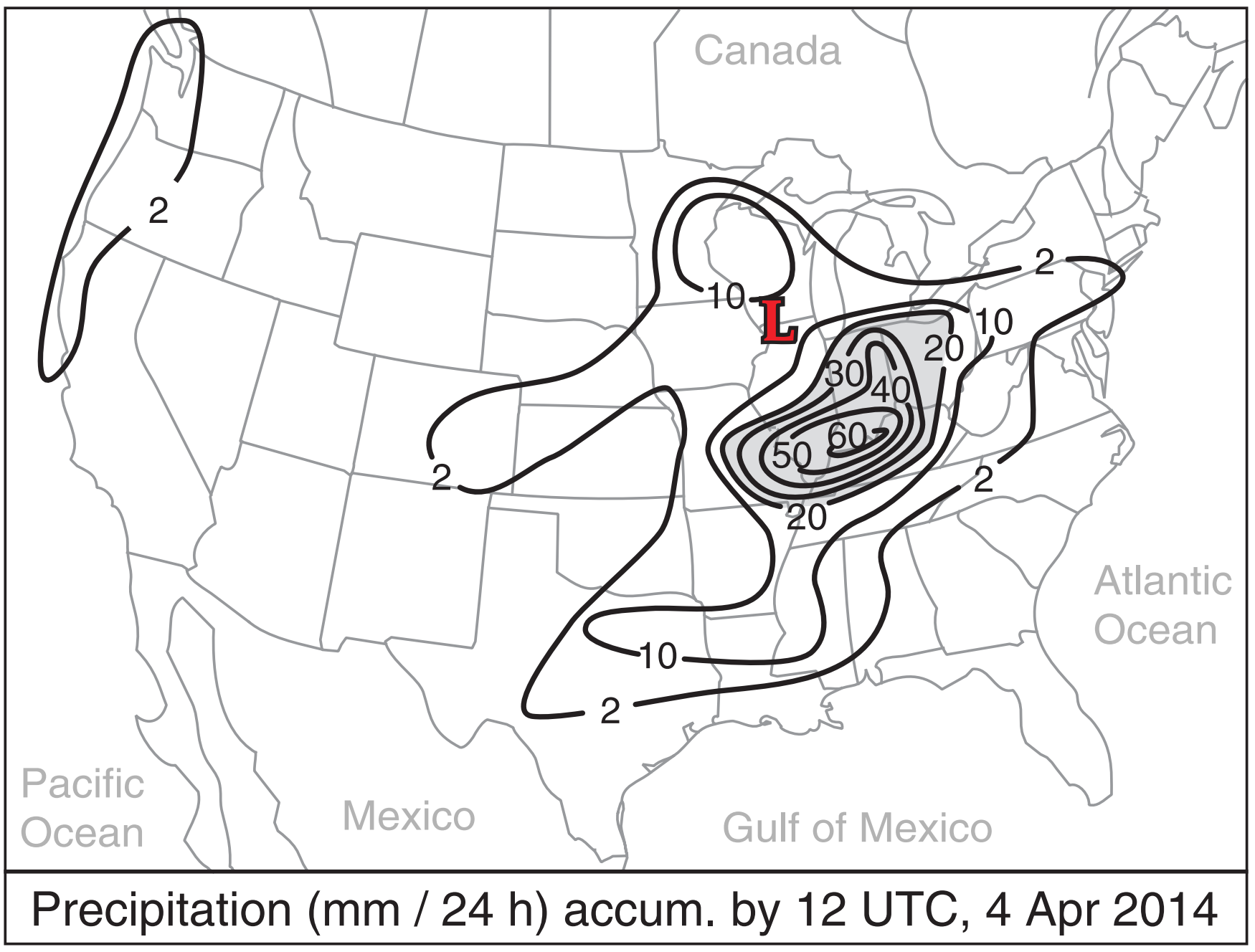
You can estimate rainfall rate with weather radar, or you can measure it with rain gauges. Fig. 13.45 shows measured precipitation liquid-equivalent depth (after melting any snow) for the case-study storm.
Sample Application
For the maximum contoured precipitation rate for the case-study storm (in Fig. 13.45), find the diabatic heating contribution to sea-level pressure tendency.
Find the Answer
Given: RR = 60 mm/24 h
Find: ∆Ps /∆t = ? kPa h–1
First, convert RR from 24 h to 1 hr: RR = 2.5 mm h–1
Use eq. (13.40): ∆Ps /∆t = –(0.082 kPa/mmrain)·(2.5 mm h–1) = –0.205 kPa h–1
Check: Physics, magnitude & units are reasonable.
Exposition: This deepening rate corresponds to 4.9 kPa day–1 — large enough to be classified as a cyclone “bomb”.
13.6.3. Net Pressure Tendency
The previous heuristic models for horizontal advection (horiz. adv.) and boundary-layer pumping (B.L.Pumping) and upper-level divergence (U.L. Diverg.) and latent heating can be combined within the framework of Fig. 13.46 to give an equation for sea-level net pressure tendency:
\(\ \begin{align} \frac{\Delta P_{s}}{\Delta t}=-M_{c} \frac{\Delta P_{s}}{\Delta s}+|g| \cdot \rho_{B L} \cdot W_{B L}-|g| \cdot \rho_{m i d} \cdot W_{m i d}-b \cdot R R\tag{13.41}\end{align}\)
tendency \(=\) horiz. adv. \(\mathcal{E}\) B.L.Pumping \(\mathcal{E}\) U.L.Diverg. \(\mathcal{E}\) heating
where (ρBL, ρmid) and (WBL, Wmid) are the average air densities and vertical velocities at boundary-layer top and mid-troposphere, respectively. The air-column horizontal translation speed is Mc (defined as positive for the average movement direction along path s). RR is rainfall rate at the surface, |g| = 9.8 m·s–2 is gravitational-acceleration magnitude, and b ≈ 0.082 kPa/mmrain. Cyclogenesis occurs when ∆Ps /∆t is negative.
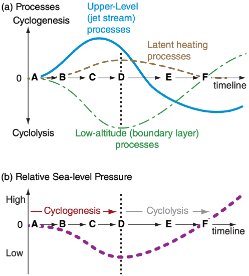
We can create a toy model of cyclone evolution using the equation above. Initially (time A in Fig. 13.47a) there is no extratropical cyclone. But if there is a Rossby wave in the jet stream, then we can anticipate horizontal divergence aloft (at the altitude of the tropopause) at a horizontal location east of the upper-level trough. As this upper-level divergence removes air molecules from the air column underneath it, sea-level pressure begins to decrease (time B in Fig. 13.47).
But once a low-pressure center forms near the surface, the combination of pressure-gradient force, Coriolis force, and frictional drag start to create a boundary-layer gradient wind that spirals into towards the low. The resulting inflow and boundary-layer pumping tends to fill (weaken) the low. So the only way the cyclone can continue to intensify is if the upper-level divergence in the jet stream is greater than the convergence in the boundary layer (times B to C in Fig. 13.47). At this time, cyclogenesis continues and sea-level pressure continues to drop.
Rising air in the cyclone (Fig. 13.46) cools adiabatically, eventually creating clouds and precipitation. The condensation creates diabatic heating, which enhances buoyancy to create faster updrafts and continued cyclogenesis (time C in Fig. 13.47).
Recall from Fig. 13.3 that circulation of air masses around the cyclone center reduces the horizontal temperature gradients there, leaving the strongest temperature gradients eastward and equatorward of the low center. Because these temperature gradients are what drives the jet-stream via the thermalwind, it means that the Rossby wave shifts eastward relative to the low center (times C to D in Fig. 13.47).
Latent heating in the cloudy updrafts continues to support cyclogenesis. Meanwhile, the upper-level divergence of the jet stream decreases. Eventually the sum of upper-level divergence and diabatic processes is insufficient to counterbalance the continued boundary-layer pumping. At this point (time D in Fig. 13.47), cyclogenesis ceases, and the sea-level pressure stops dropping. The cyclone has reached its mature stage and is still strong (low surface pressures, strong winds, heavy precipitation), but will not be getting stronger.
The strong circulation around the low continues to cause strong boundary-layer pumping, which ceaselessly tends to weaken the cyclone. Without the jet-stream support aloft, the air column begins to fill with molecules — cyclolysis has begun.
As the cyclone occludes (Figs. 13.3e & f), the Rossby wave shifts so far eastward that the jet-stream is causing upper-level convergence over the weakening low (time E in Fig. 13.47), thereby helping to fill it even faster with air molecules.
Eventually, the central pressure rises to equal the surrounding pressures (i.e., no horizontal pressure gradient). Winds decrease, condensation and precipitation end, and the circulation spins down. By time F in Fig. 13.47, the cyclone has disappeared, and anticyclogenesis (creation of surface high-pressure) has begun.
During the approximately three-day life cycle, the cyclone acted to move cold air equatorward and warm air poleward to reduce the baroclinic instability that had created it (as per Le Chatelier’s principle).
Sample Application
A cyclone experiences the following processes:
- Rainfall of 2 mm h–1.
- Advection due to a 15 m/s west wind across a horizontal gradient of ∆P/∆x of 0.5 kPa/300 km.
- Upper-level divergence causing Wmid = 0.04 m s–1 .
- Boundary-layer pumping WBL = 0.02 m s–1 .
Given: ρmid ≈ 0.5 kg·m–3 , ρBL ≈ 1.112 kg·m–3
What is the sea-level pressure tendency?.
Find the Answer
Given: ∆P/∆s = 0.5 kPa/300 km, RR = 2 mm h–1 , Wmid = 0.02 m s–1, WBL = 0.02 m s–1,
Find: ∆Ps /∆t = ? kPa h–1
Apply eq. (13.41): ∆Ps /∆t =
\(-\left(15 \frac{\mathrm{m}}{\mathrm{s}}\right)\left(\frac{0.5 \mathrm{kPa}}{3 \times 10^{5} \mathrm{m}}\right)+\left(9.8 \frac{\mathrm{m}}{\mathrm{s}^{2}}\right)\left(1.112 \frac{\mathrm{kg}}{\mathrm{m}^{3}}\right)\left(0.02 \frac{\mathrm{m}}{\mathrm{s}}\right)-\left(9.8 \frac{\mathrm{m}}{\mathrm{s}^{2}}\right)\left(0.5 \frac{\mathrm{kg}}{\mathrm{m}^{3}}\right)\left(0.04 \frac{\mathrm{m}}{\mathrm{s}}\right)-\left(0.084 \frac{\mathrm{kPa}}{\mathrm{mm}}\right)\left(2 \frac{\mathrm{mm}}{\mathrm{h}}\right)\)
∆Ps /∆t = (–2.5 + 21.8 – 19.6 – 4.7 )x10–5 kPa s–1
tendency = horiz. adv. & B.L.Pumping & U.L.Diverg. & heating
= – 5 x10⁻⁵ kPa s–1 = – 0.18 kPa h–1
Check: Physics, magnitude & units are reasonable.
Exposition: The negative sign implies cyclogenesis. In the B.L.pumping and U.L.Diverg. terms I divided by 1000 to convert Pa into kPa. For the rainfall term I converted from kPa h–1 to kPa s–1.


