11.9: Types of Vorticity

11.9.1. Relative-vorticity Definition

Counterclockwise rotation about a local vertical axis defines positive vorticity. One type of vorticity ζ_r , called relative vorticity, is measured relative to both the location of the object and to the surface of the Earth (also see the Forces & Winds chapter).

Figure 11.42 Flower blossoms dropped into a river illustrate positive relative vorticity (counterclockwise rotation) caused by river-current shear as the blossoms translate downstream.

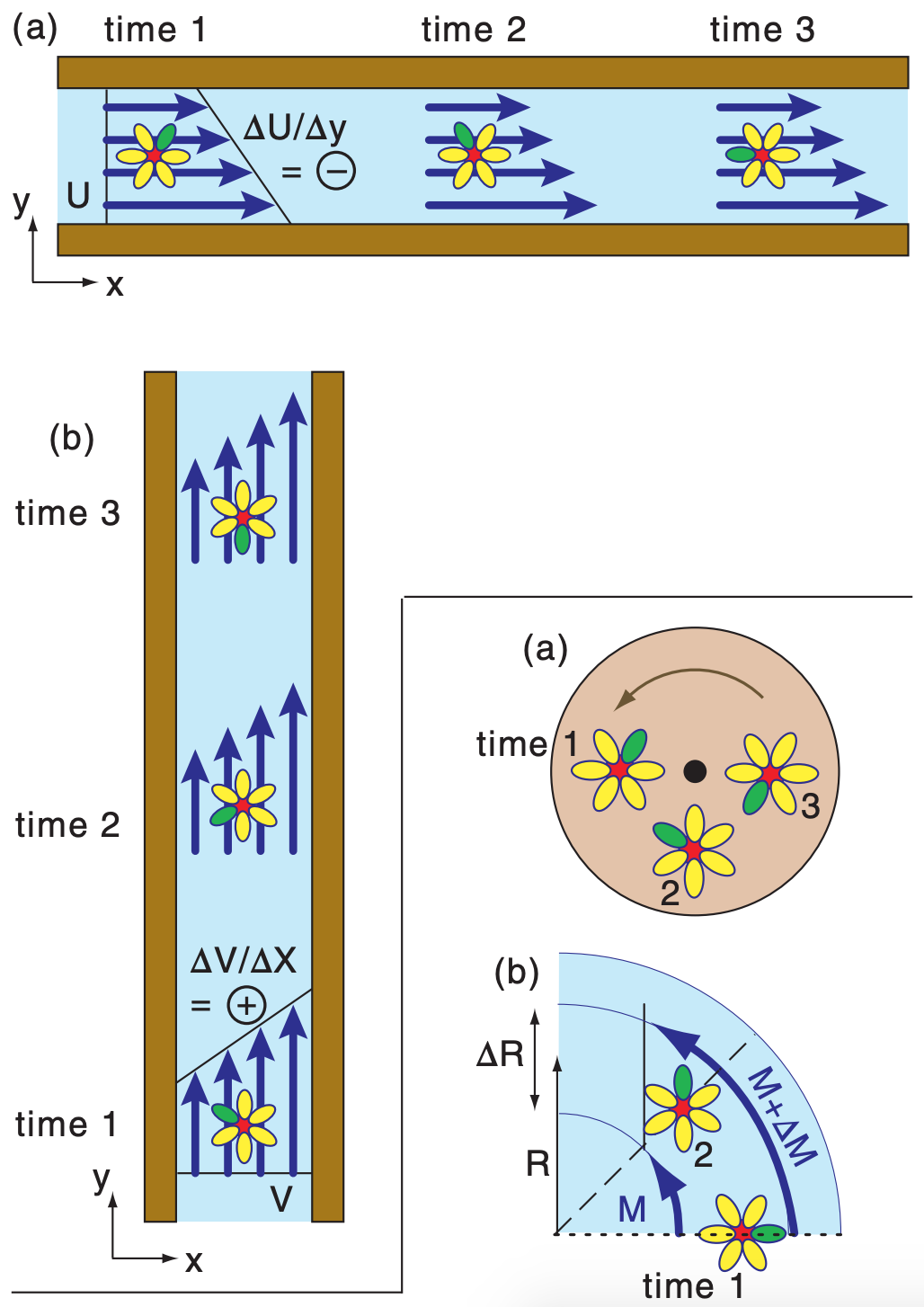
Figure 11.43 (a) Vorticity associated with solid-body rotation, illustrated with a flower blossom glued to a solid turntable at time 1. (b) Vorticity caused by radial shear of tangential velocity M.

Picture a flower blossom dropped onto a straight river, where the river current has shear (Fig. 11.42). As the floating blossom drifts (translates) downstream, it also spins due to the velocity shear of the current. Both Figs. 11.42a & b show counterclockwise rotation, giving positive relative vorticity as defined by:

\(\ \begin{align} \zeta_{r}=\frac{\Delta V}{\Delta x}-\frac{\Delta U}{\Delta y}\tag{11.20}\end{align}\)

for (U, V) positive in the local (x, y) directions.

Next, consider a flower blossom glued to a solid turntable, as sketched in Fig. 11.43a. As the table turns, so does the orientation of the flower petals relative to the center of the flower. This is shown in Fig. 11.43b. Solid-body rotation requires vectors that start on the dotted line and end on the dashed line. But in a river (or atmosphere), currents can have additional radial shear of the tangential velocity M. Thus, relative vorticity can also be defined as:

\(\ \begin{align} \zeta_{r}=\frac{\Delta M}{\Delta R}+\frac{M}{R}\tag{11.21}\end{align}\)

Figure 11.44 Weather map example of relative vorticity (contour lines, with units of 10^–5 s^–1) near the tropopause (at the 20 kPa isobaric surface) at 12 UTC on 5 January 2001. White arrows show jet stream axis of fastest winds over North America and the Atlantic Ocean. Shading gives wind speeds every 10 m s^–1 from 30 m s^–1 (lightest grey) to over 80 m s^–1 (darkest grey). (Based on NCEP/NCAR 40-year reanalysis data, utilizing the plotting tool by Christopher Godfrey, the Univ. of Oklahoma School of Meteorology.)

INFO • Solid Body Relative Vorticity

To get eq. (11.22) you can begin with eq. (11.21):

\(\zeta_{r}=\frac{\Delta M}{\Delta R}+\frac{M}{R}\)

For solid-body rotation, ∆M/∆R exactly equals M/R, as is illustrated in the time 1 2 M+∆M M=0 R ∆R figure at right. Hence:

\(\zeta_{r}=\frac{(M-0)}{R}+\frac{M}{R}=\frac{2 M}{R}\)

which is eq. (11.22).

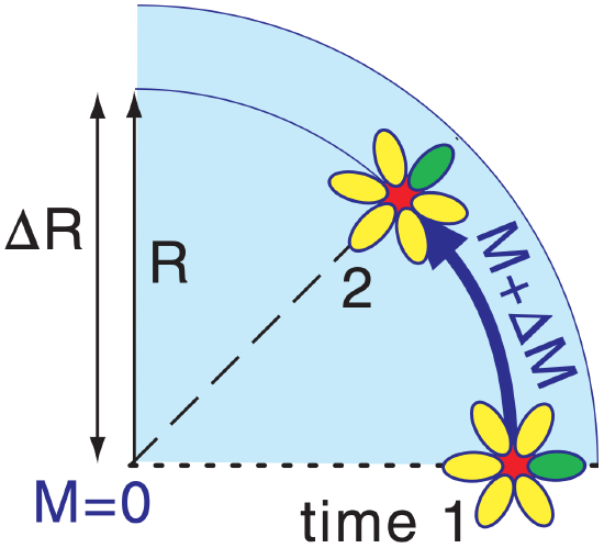
For pure solid-body rotation (where the tangential current- or wind-vectors do indeed start at the same dotted line and end at the same dashed line in Fig. 11.43b), eq. (11.21) can be rewritten as

\(\ \begin{align} \zeta_{r}=\frac{2 M}{R}\tag{11.22}\end{align}\)

Relative vorticity has units of s–1. A quick way to determine the sign of the vorticity is to curl the fingers of your right hand in the direction of rotation. If your thumb points up, then vorticity is positive. This is the right-hand rule. Fig. 11.44 shows relative vorticity of various signs, where vorticity was created by both shear and curvature.

Sample Application

At 50°N is a west wind of 100 m s^–1. At 46°N is a west wind of 50 m s^–1. Find the (a) relative, & (b) absolute vorticity

Find the Answer

Given: U₂ =100 m s^–1, U1 =50 m s^–1, ∆ϕ =4°lat. V =0

Find: ζ _r = ? s^–1 , ζ _a = ? s^–1

(a) Use eq. (11.20): Appendix A: 1°latitude = 111 km ζ _r = – (100 – 50 m s^–1) / (4.4x10⁵ m) = –1.14x10^–4 s^–1

(b) Average ϕ = 48°N. Thus, f_c = (1.458x10^–4 s^–1)·sin(48°)

f_c = 1.08x10^–4 s^–1. then, use eq. (11.23):

ζ_a = (–1.14x10^–4) + (1.08x10^–4) = –6x10^–6 s^–1 .

Check: Physics and units are reasonable.

Exposition: Shear vorticity from a strong jet stream, but its vorticity is opposite to the Earth’s rotation.

Sample Application

Given a N. Hemisphere high-pressure center with tangential winds of 5 m s^–1 at radius 500 km. What is the value of relative vorticity?

Find the Answer

Given: |M|= 5 m s^–1 (anti-cyclonic), R = 500,000 m.

Find: ζ _r = ? s^–1

In the N. Hem., anti-cyclonic winds turn clockwise, so using the right-hand rule means your thumb points down, so vorticity will be negative. Apply eq. (11.22):

ζ _r = – 2 · (5 m s^–1) / (5x10⁵ m) = –2x10^–5 s^–1

Check: Physics and units are reasonable.

Exposition: Anticyclones often have smaller magnitudes of relative vorticity than cyclones (Fig. 11.44).

11.9.2. Absolute-vorticity Definition

Define an absolute vorticity ζ_a as the sum of the vorticity relative to the Earth plus the rotation of the Earth relative to the so-called fixed stars:

\(\ \begin{align} \zeta_{a}=\zeta_{r}+f_{c}\tag{11.23}\end{align}\)

where f_c = 2Ω·sin(ϕ) is the Coriolis parameter, 2Ω = 1.458x10^–4 s^–1 is the angular velocity of the Earth relative to the fixed stars, and latitude is ϕ. Absolute vorticity has units of s^–1.

11.9.3. Potential-vorticity Definition

Define a potential vorticity ζ _p as absolute vorticity per unit depth ∆z of the rotating air column:

\(\ \begin{align} \zeta_{p}=\frac{\zeta_{r}+f_{c}}{\Delta z}= constant \tag{11.24}\end{align}\)

This is the most important measure of vorticity because it is constant (i.e., is conserved) for flows having no latent or radiative heating, and no turbulent drag. Potential vorticity units are m^–1 s^–1.

Sample Application

A hurricane at latitude 20°N has tangential winds of 50 m s^–1 at radius 50 km from the center averaged over a 15 km depth. Find potential vorticity, assuming solid-body rotation for simplicity.

Find the Answer

Assume the shear is in the cyclonic direction.

Given: ∆z = 15,000 m, ϕ = 20°N, M = 50 m s^–1, ∆R = 50,000 m.

Find: ζ_p = ? m^–1·s^–1

Apply eqs. (11.22) with (11.24):

\(\zeta_{p}=\frac{\frac{2 \cdot(50 \mathrm{m} / \mathrm{s})}{5 \times 10^{4} \mathrm{m}}+\left(1.458 \times 10^{-4} \mathrm{s}^{-1}\right) \cdot \sin \left(20^{\circ}\right)}{15000 \mathrm{m}}\)

= (2x10^–3+5x10^–5 )/15000 m = 1.37x10^–7 m^–1·s^–1

Check: Physics & units are reasonable.

Exposition: Positive sign due to cyclonic rotation.

Rewrite the potential vorticity using eqs. (11.24 & 11.21):

\(\ \begin{align} \frac{\Delta M}{\Delta R}+\frac{M}{R} \quad+f_{c}=\zeta_{p} \cdot \Delta z\tag{11.25}\end{align}\)
shear curvature planetary stretching

The initial values of absolute vorticity and rotatingair depth determine the value for the constant ζ_p. In order to preserve the equality in the equation above while preserving the constant value of ζ_p, any increase of depth ∆z of the rotating layer of air must be associated with greater relative vorticity (air spins faster) or larger f_c (rotating air moves poleward).

11.9.4. Isentropic Potential Vorticity Definition

By definition, an isentropic surface connects locations of equal entropy. But non-changing entropy corresponds to non-changing potential temperature θ in the atmosphere (i.e., adiabatic conditions). If you calculate the absolute vorticity (ζ_r + f_c) on such a surface, then it can be used to define an isentropic potential vorticity (IPV):

\(\ \begin{align} \zeta_{I P V}=\frac{\zeta_{r}+f_{c}}{\rho} \cdot\left(\frac{\Delta \theta}{\Delta z}\right)=\frac{\zeta_{a}}{\rho} \cdot\left(\frac{\Delta \theta}{\Delta z}\right)\tag{11.26}\end{align}\)

or

\(\ \begin{align} \zeta_{I P V}=-|g| \cdot\left(\zeta_{r}+f_{c}\right) \cdot \frac{\Delta \theta}{\Delta p}\tag{11.27}\end{align}\)

where air pressure is p, air density is ρ , gravitational acceleration magnitude is |g|, and ∆θ/∆z indicates the static stability.

Sample Application

If ζ_a = 1.5x10^–4 s^–1, ρ = 0.7 kg m^–3 and ∆θ/∆z = 4 K km^–1, find the isentropic potential vorticity in PVU.

Find the Answer

Given: ζ_a = 1.5x10^–4 s^–1, ρ = 0.7 kg m^–3 , ∆θ/∆z = 4 K km^–1

Find: ζ_IPV = ? PVU

Apply eq. (11.26):

\(\begin{aligned} \zeta_{I P V} &=\frac{\left(1.5 \times 10^{-4} \mathrm{s}^{-1}\right)}{\left(0.7 \mathrm{kg} \cdot \mathrm{m}^{-3}\right)} \cdot\left(4 \mathrm{K} \cdot \mathrm{km}^{-1}\right)=8.57 \times 10^{-7} \mathrm{Km}^{2} \cdot \mathrm{s}^{-1} \cdot \mathrm{kg}^{-1}=\underline{0.857} \mathrm{PVU} \end{aligned}\)

Check: Physics & units are reasonable.

Exposition: As expected for tropospheric air, the answer has magnitude less than 1.5 PVU.

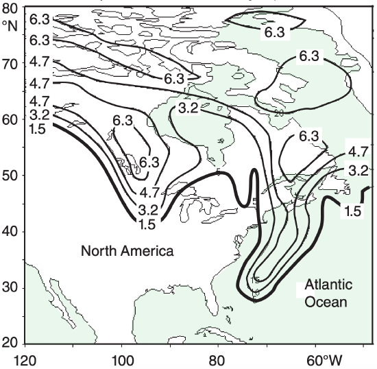
Define a potential vorticity unit (PVU) such that 1 PVU = 10^–6 K·m²·s^–1·kg^–1. The stratosphere has lower density and greater static stability than the troposphere, hence stratospheric air has IPV values that are typically 100 times larger than for tropospheric air. Typically, ζ_IPV > 1.5 PVU for stratospheric air (a good atmospheric cross-section example is shown in the Extratropical Cyclone chapter).

For idealized situations where the air moves adiabatically without friction while following a constant θ surface (i.e., isentropic motion), then ζ_IPV is conserved, which means you can use it to track air motion. Also, stratospheric air does not instantly lose its large IPV upon being mixed downward into the troposphere.

Figure 11.45 Example of isentropic potential vorticity on the 315 K isentropic surface, at 00 UTC on 5 January 2001. Units are PVU. Values greater than 1.5 are in stratospheric air. Because the tropopause is at lower altitude near the poles than at the equator, the 315 K potential temperature surface crosses the tropopause; so it is within the troposphere in the southern part of the figure and in the stratosphere in the northern part. Tropopause folds are evident by the high PVU values just west of the Great Lakes, and just east of the North American coastline. (Based on NCEP/ NCAR 40-year reanalysis data, with initial plots produced using the plotting tool by Christopher Godfrey, the University of Oklahoma School of Meteorology.)

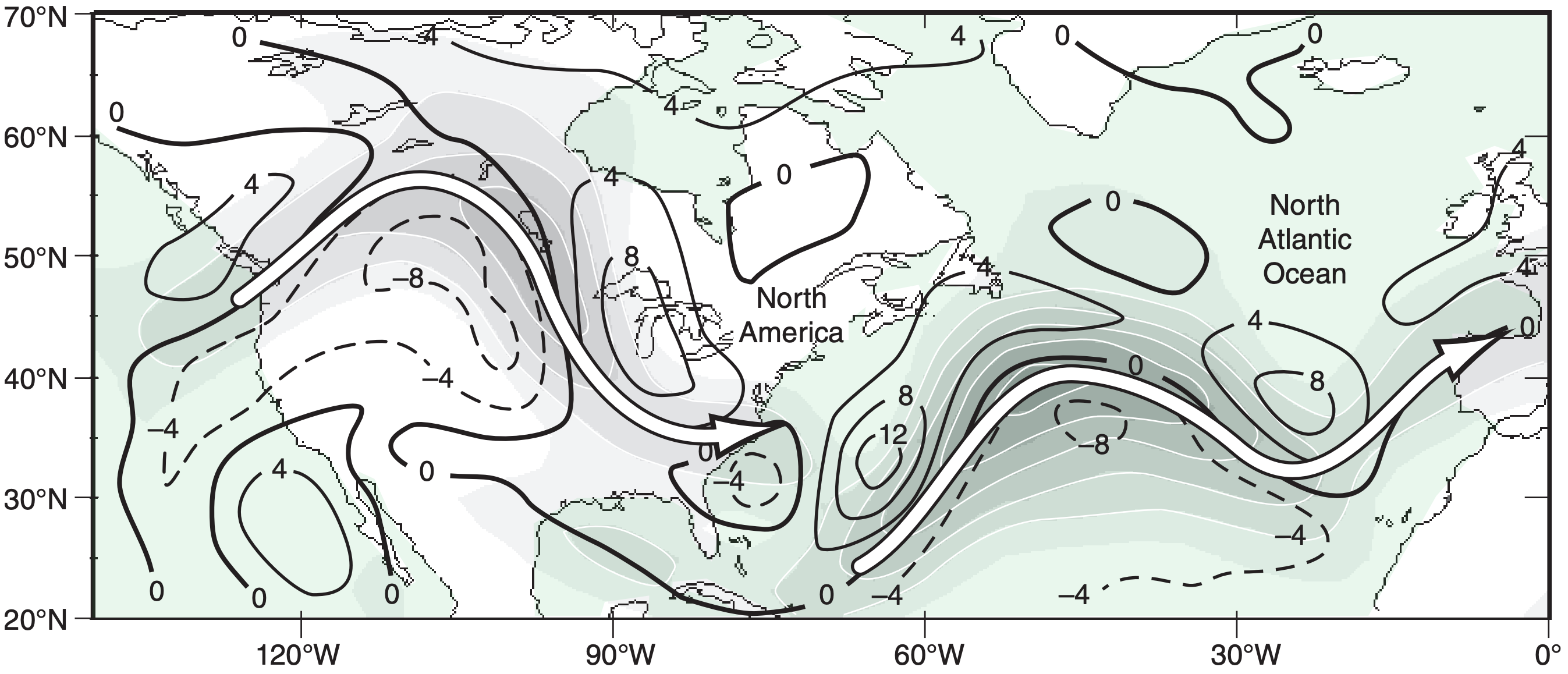
Thus, IPV is useful for finding tropopause folds and the accompanying intrusions of stratospheric air into the troposphere (Fig. 11.45), which can bring down toward the ground the higher ozone concentrations and radionuclides (radioactive atoms from former atomic-bomb tests) from the stratosphere.

Because isentropic potential vorticity is conserved, if static stability (∆θ/∆z) weakens, then eq. (11.26) says absolute vorticity must increase to maintain constant IPV. For example, Fig. 11.46 shows isentropes for flow from west to east across the Rocky Mountains. Where isentropes are spread far apart, static stability is low. Because air tends to follow isentropes (for frictionless adiabatic flow), a column of air between two isentropes over the crest of the Rockies will remain between the same two isentropes as the air continues eastward.

Figure 11.46 Wind blowing from west to east (A) over the Rocky Mountains creates mountain waves and downslope winds, which cause greater separation (B) between the 302 and 310 K isentropes to the lee of the mountains. This greater separation implies reduced static stability and vertical stretching.

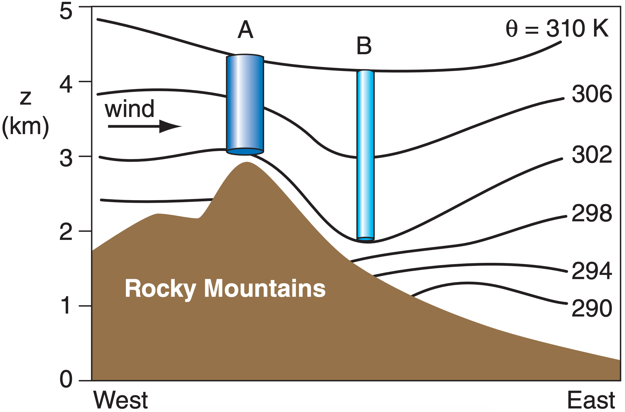
Thus, the column of air shown in Fig. 11.46 becomes stretched on the lee side of the Rockies and its static stability decreases (same ∆θ, but spread over a larger ∆z). Thus, absolute vorticity in the stretched region must increase. Such increased cyclonic vorticity encourages formation of low-pressure systems (extratropical cyclones) to the lee of the Rockies — a process called lee cyclogenesis.

Sample Application

Given Fig. 11.46. (a) Estimate ∆θ/∆z at A and B. (b) if the initial absolute vorticity at A is 10^–4 s^–1, find the absolute vorticity at B.

Find the Answer

Given: ζ_a = 10^–4 s^–1 at A, θ_top = 310 K, θ_bottom = 302 K.

Find: (a) ∆θ/∆z = ? K km^–1 at A and B.

(b) ζ_a = ? s^–1 at B.

∆θ = 310 K – 302 K = 8 K at A & B. Estimate the altitudes at the top and bottom of the cylinders in Fig. 11.46.

A: z_top = 4.4 km, z_bottom = 3.1 km. Thus ∆z_A = 1.3 km.

B: z_top = 4.2 km, z_bottom = 1.9 km. Thus ∆z_B = 2.3 km.

(a) ∆θ/∆z = 8K / 1.3 km = 6.15 K km^–1 at A

∆θ/∆z = 8K / 2.3 km = 3.48 K km^–1 at B.

(b) If initial (A) and final (B) IPV are equal, then rearranging eq. (11.26) and substituting (ζ_r + f_c) = ζ_a gives:

ζ_aB = ζ_aA · (∆z_B/∆z_A) = (10^–4 s )·[(2.3 km)/(1.3 km)] = 1.77x 10^–4 s^–1

Check: Sign, magnitude & units are reasonable.

Exposition: Static stability ∆θ/∆z is much weaker at B than A. Thus absolute vorticity at B is much greater than at A. If the air flow directly from west to east and if the initial relative vorticity were zero, then the final relative vorticity is ζ_r = 0.77x10^–4 s^–1. Namely, to the lee of the mountains, cyclonic rotation forms in the air where none existed upwind. Namely, this implies cyclogenesis (birth of cyclones) to the lee (downwind) of the Rocky Mountains.