11.13: Ekman Spiral of Ocean Currents

Frictional drag between the atmosphere and ocean enables winds to drive ocean-surface currents. Coriolis force causes the surface current to be 45° to the right of the wind direction in the Northern Hemisphere. Drag between that surface-current and deeper water drives deeper currents that are slower, and which also are to the right of the current above. The result is an array of ocean-current vectors that trace a spiral (Fig. 11.61) called the Ekman spiral.

Figure 11.61 Example of an Ekman spiral in the ocean. Blue arrows show ocean currents at different depths (numbers in green). U current direction is aligned with the near-surface wind direction. Red arrow shows the wind direction, but speed is much greater. This example is based on a 10 m s^–1 wind at 45° latitude.

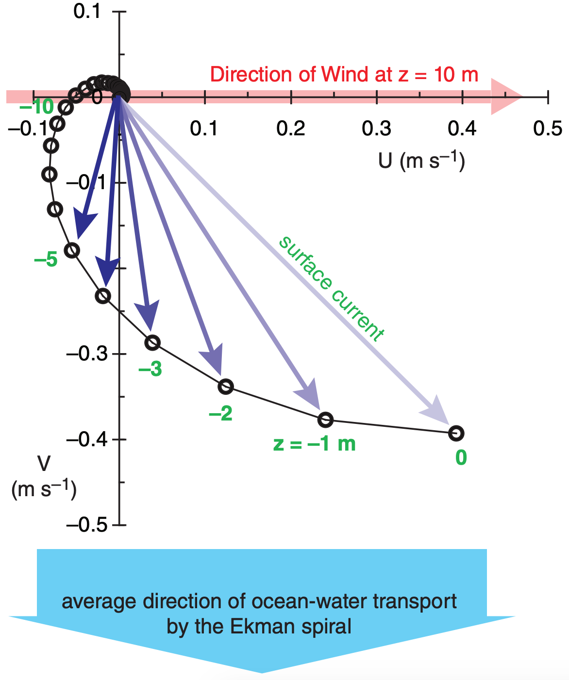
The equilibrium horizontal ocean-current components (U, V, for a rotated coordinate system having U aligned with the wind direction) as a function of depth (z) are:

\(\ \begin{align} U=\left[\frac{u_{*} \operatorname{water}^{2}}{\left(K \cdot f_{c}\right)^{1 / 2}}\right] \cdot\left[e^{z / D} \cdot \cos \left(\frac{z}{D}-\frac{\pi}{4}\right)\right]\tag{11.52a}\end{align}\)

\(\ \begin{align} V=\left[\frac{u_{*} w a t e r^{2}}{\left(K \cdot f_{c}\right)^{1 / 2}}\right] \cdot\left[e^{z / D} \cdot \sin \left(\frac{z}{D}-\frac{\pi}{4}\right)\right]\tag{11.52b}\end{align}\)

where z is negative below the ocean surface, f_c = Coriolis parameter, and u_*water is a friction velocity (m s^–1) for water. It can be found from

\(\ \begin{align} u_{*water}^{2}=\frac{\rho_{a i r}}{\rho_{\text {water}}} \cdot u_{* a i r}^{2}\tag{11.53}\end{align}\)

where the density ratio ρ_air/ρ_water ≈ 0.001195 for sea water. The friction velocity (m s–1) for air can be approximated using Charnock’s relationship:

\(\ \begin{align} u_{* a i r}^{2} \approx 0.00044 \cdot M^{2.55}\tag{11.54}\end{align}\)

where M is near-surface wind speed (at z = 10 m) in units of m s^–1.

The Ekman-layer depth scale is

\(\ \begin{align} D=\sqrt{\frac{2 \cdot K}{f_{c}}}\tag{11.55}\end{align}\)

where K is the ocean eddy viscosity (a measure of ability of ocean turbulence to mix momentum). One approximation is K ≈ 0.4 |z| u_*water . Although K varies with depth, for simplicity in this illustration I used constant K corresponding to its value at z = –0.2 m, which gave K ≈ 0.001 m² s^–1.

The average water-mass transport by Ekman ocean processes is 90° to the right (left) of the near-surface wind in the N. (S.) Hemisphere (Fig. 11.61). This movement of water affects sea-level under hurricanes (see the Tropical Cyclone chapter).

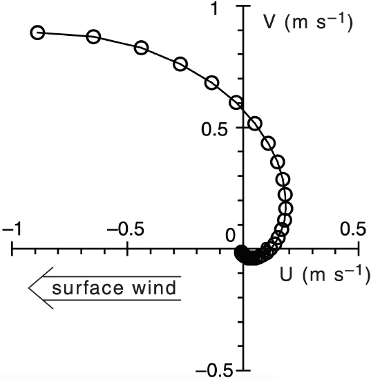
Sample Application

For an east wind of 14 m/s at 30°N, graph the Ekman spiral.

Find the Answer

Given: M = 14 m·s^–1, ϕ = 30°N

Find: [U , V ] (m s^–1) vs. depth z (m)

Using a relationship from the Forces and Winds chapter, find the Coriolis parameter: f_c = 7.29x10^–5 s^–1 .

Next, use Charnock’s relationship. eq. (11.54): u_*air² = 0.00044 (14 ^2.55) = 0.368 m² s^–2 .

Then use eq. (11.53):

u_*water² = 0.001195 · (0.368 m² s^–2) = 0.00044 m² s^–2

Estimate K at depth 0.2 m in the ocean from

K ≈ 0.4 · (0.2 m) ·[0.00044 m² s^–2] ^1/2 = 0.00168 m² s^–1

Use eq. (11.55):

D = [2 · (0.00168 m² s^–1) / (7.29x10^–5 s^–1) ]^1/2 = 6.785 m

Use a spreadsheet to solve for (U, V) for a range of z, using eqs. (11.52). I used z = 0, –1, –2, –3 m etc.

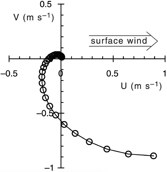
Finally, rotate the graph 180° because the wind is from the East.

Check: Physics & units are reasonable.

Exposition: Net transport of ocean water is toward the north for this East wind case.