11.5: Geostrophic Wind and Geostrophic Adjustment
- Page ID
- 9600
\( \newcommand{\vecs}[1]{\overset { \scriptstyle \rightharpoonup} {\mathbf{#1}} } \)
\( \newcommand{\vecd}[1]{\overset{-\!-\!\rightharpoonup}{\vphantom{a}\smash {#1}}} \)
\( \newcommand{\id}{\mathrm{id}}\) \( \newcommand{\Span}{\mathrm{span}}\)
( \newcommand{\kernel}{\mathrm{null}\,}\) \( \newcommand{\range}{\mathrm{range}\,}\)
\( \newcommand{\RealPart}{\mathrm{Re}}\) \( \newcommand{\ImaginaryPart}{\mathrm{Im}}\)
\( \newcommand{\Argument}{\mathrm{Arg}}\) \( \newcommand{\norm}[1]{\| #1 \|}\)
\( \newcommand{\inner}[2]{\langle #1, #2 \rangle}\)
\( \newcommand{\Span}{\mathrm{span}}\)
\( \newcommand{\id}{\mathrm{id}}\)
\( \newcommand{\Span}{\mathrm{span}}\)
\( \newcommand{\kernel}{\mathrm{null}\,}\)
\( \newcommand{\range}{\mathrm{range}\,}\)
\( \newcommand{\RealPart}{\mathrm{Re}}\)
\( \newcommand{\ImaginaryPart}{\mathrm{Im}}\)
\( \newcommand{\Argument}{\mathrm{Arg}}\)
\( \newcommand{\norm}[1]{\| #1 \|}\)
\( \newcommand{\inner}[2]{\langle #1, #2 \rangle}\)
\( \newcommand{\Span}{\mathrm{span}}\) \( \newcommand{\AA}{\unicode[.8,0]{x212B}}\)
\( \newcommand{\vectorA}[1]{\vec{#1}} % arrow\)
\( \newcommand{\vectorAt}[1]{\vec{\text{#1}}} % arrow\)
\( \newcommand{\vectorB}[1]{\overset { \scriptstyle \rightharpoonup} {\mathbf{#1}} } \)
\( \newcommand{\vectorC}[1]{\textbf{#1}} \)
\( \newcommand{\vectorD}[1]{\overrightarrow{#1}} \)
\( \newcommand{\vectorDt}[1]{\overrightarrow{\text{#1}}} \)
\( \newcommand{\vectE}[1]{\overset{-\!-\!\rightharpoonup}{\vphantom{a}\smash{\mathbf {#1}}}} \)
\( \newcommand{\vecs}[1]{\overset { \scriptstyle \rightharpoonup} {\mathbf{#1}} } \)
\( \newcommand{\vecd}[1]{\overset{-\!-\!\rightharpoonup}{\vphantom{a}\smash {#1}}} \)
\(\newcommand{\avec}{\mathbf a}\) \(\newcommand{\bvec}{\mathbf b}\) \(\newcommand{\cvec}{\mathbf c}\) \(\newcommand{\dvec}{\mathbf d}\) \(\newcommand{\dtil}{\widetilde{\mathbf d}}\) \(\newcommand{\evec}{\mathbf e}\) \(\newcommand{\fvec}{\mathbf f}\) \(\newcommand{\nvec}{\mathbf n}\) \(\newcommand{\pvec}{\mathbf p}\) \(\newcommand{\qvec}{\mathbf q}\) \(\newcommand{\svec}{\mathbf s}\) \(\newcommand{\tvec}{\mathbf t}\) \(\newcommand{\uvec}{\mathbf u}\) \(\newcommand{\vvec}{\mathbf v}\) \(\newcommand{\wvec}{\mathbf w}\) \(\newcommand{\xvec}{\mathbf x}\) \(\newcommand{\yvec}{\mathbf y}\) \(\newcommand{\zvec}{\mathbf z}\) \(\newcommand{\rvec}{\mathbf r}\) \(\newcommand{\mvec}{\mathbf m}\) \(\newcommand{\zerovec}{\mathbf 0}\) \(\newcommand{\onevec}{\mathbf 1}\) \(\newcommand{\real}{\mathbb R}\) \(\newcommand{\twovec}[2]{\left[\begin{array}{r}#1 \\ #2 \end{array}\right]}\) \(\newcommand{\ctwovec}[2]{\left[\begin{array}{c}#1 \\ #2 \end{array}\right]}\) \(\newcommand{\threevec}[3]{\left[\begin{array}{r}#1 \\ #2 \\ #3 \end{array}\right]}\) \(\newcommand{\cthreevec}[3]{\left[\begin{array}{c}#1 \\ #2 \\ #3 \end{array}\right]}\) \(\newcommand{\fourvec}[4]{\left[\begin{array}{r}#1 \\ #2 \\ #3 \\ #4 \end{array}\right]}\) \(\newcommand{\cfourvec}[4]{\left[\begin{array}{c}#1 \\ #2 \\ #3 \\ #4 \end{array}\right]}\) \(\newcommand{\fivevec}[5]{\left[\begin{array}{r}#1 \\ #2 \\ #3 \\ #4 \\ #5 \\ \end{array}\right]}\) \(\newcommand{\cfivevec}[5]{\left[\begin{array}{c}#1 \\ #2 \\ #3 \\ #4 \\ #5 \\ \end{array}\right]}\) \(\newcommand{\mattwo}[4]{\left[\begin{array}{rr}#1 \amp #2 \\ #3 \amp #4 \\ \end{array}\right]}\) \(\newcommand{\laspan}[1]{\text{Span}\{#1\}}\) \(\newcommand{\bcal}{\cal B}\) \(\newcommand{\ccal}{\cal C}\) \(\newcommand{\scal}{\cal S}\) \(\newcommand{\wcal}{\cal W}\) \(\newcommand{\ecal}{\cal E}\) \(\newcommand{\coords}[2]{\left\{#1\right\}_{#2}}\) \(\newcommand{\gray}[1]{\color{gray}{#1}}\) \(\newcommand{\lgray}[1]{\color{lightgray}{#1}}\) \(\newcommand{\rank}{\operatorname{rank}}\) \(\newcommand{\row}{\text{Row}}\) \(\newcommand{\col}{\text{Col}}\) \(\renewcommand{\row}{\text{Row}}\) \(\newcommand{\nul}{\text{Nul}}\) \(\newcommand{\var}{\text{Var}}\) \(\newcommand{\corr}{\text{corr}}\) \(\newcommand{\len}[1]{\left|#1\right|}\) \(\newcommand{\bbar}{\overline{\bvec}}\) \(\newcommand{\bhat}{\widehat{\bvec}}\) \(\newcommand{\bperp}{\bvec^\perp}\) \(\newcommand{\xhat}{\widehat{\xvec}}\) \(\newcommand{\vhat}{\widehat{\vvec}}\) \(\newcommand{\uhat}{\widehat{\uvec}}\) \(\newcommand{\what}{\widehat{\wvec}}\) \(\newcommand{\Sighat}{\widehat{\Sigma}}\) \(\newcommand{\lt}{<}\) \(\newcommand{\gt}{>}\) \(\newcommand{\amp}{&}\) \(\definecolor{fillinmathshade}{gray}{0.9}\)11.5.1. Ageostrophic Winds at the Equator

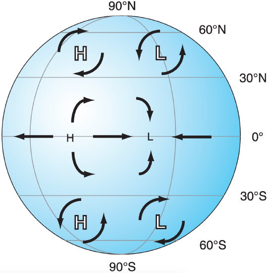
Air at the equator can move directly from high (H) to low (L) pressure (Fig. 11.18 - center part) under the influence of pressure-gradient force. Zero Coriolis force at the equator implies infinite geostrophic winds. But actual winds have finite speed, and are thus ageostrophic (not geostrophic).
Because such flows can happen very easily and quickly, equatorial air tends to quickly flow out of highs into lows, causing the pressure centers to neutralize each other. Indeed, weather maps at the equator show very little pressure variations zonally. One exception is at continent-ocean boundaries, where continental-scale differential heating can continually regenerate pressure gradients to compensate the pressure-equalizing action of the wind. Thus, very small pressure gradients can cause continental-scale (5000 km) monsoon circulations near the equator. Tropical forecasters focus on winds, not pressure.
If the large-scale pressure is uniform in the horizontal near the equator (away from monsoon circulations), then the horizontal pressure gradients disappear. With no horizontal pressure-gradient force, no large-scale winds can be driven there. However, winds can exist at the equator due to inertia — if the winds were first created geostrophically at nonzero latitude and then coast across the equator.
But at most other places on Earth, Coriolis force deflects the air and causes the wind to approach geostrophic or gradient values (see the Forces & Winds chapter). Non-accelerating geostrophic and gradient winds do not cross isobars, so they cannot transfer mass from highs to lows. Thus, significant pressure patterns (e.g., strong high and low centers, Fig. 11.18) can be maintained for long periods at mid-latitudes in the global circulation.
11.5.2. Definitions
“Like other exploratory processes, [the scientific method] can be resolved into a dialogue between fact and fancy, the actual and the possible; between what could be true and what is in fact the case. The purpose of scientific enquiry is not to compile an inventory of factual information, nor to build up a totalitarian world picture of Natural Laws in which every event that is not compulsory is forbidden. We should think of it rather as a logically articulated structure of justifiable beliefs about a Possible World — a story which we invent and criticize and modify as we go along, so that it ends by being, as nearly as we can make it, a story about real life.”
- by Nobel Laureate Sir Peter Medawar (1982) Pluto’s Republic. Oxford Univ. Press.
A temperature field is a map showing how temperatures are spatially distributed. A wind field is a map showing how winds are distributed. A mass field represents how air mass is spatially distributed. But we don’t routinely measure air mass.
In the first Chapter, we saw how pressure at any one altitude depends on (is a measure of) all the air mass above that altitude. So we can use the pressure field at a fixed altitude as a surrogate for the mass field. Similarly, the height field on a map of constant pressure is another surrogate.
But the temperature and mass fields are coupled via the hypsometric equation (see Chapter 1).
Namely, if the temperature changes in the horizontal (defined as a baroclinic atmosphere), then pressures at any fixed altitude must also change in the horizontal. Later in this chapter, we will also see how the wind and temperature fields are coupled (via the thermal wind relationship).
11.5.3. Geostrophic Adjustment - Part 1

The tendency of non-equatorial winds to approach geostrophic values (or gradient values for curved isobars) is a very strong process in the Earth’s atmosphere. If the actual winds are not in geostrophic balance with the pressure patterns, then both the winds and the pressure patterns tend to change to bring the winds back to geostrophic (another example of Le Chatelier’s Principle). Geostrophic adjustment is the name for this process.
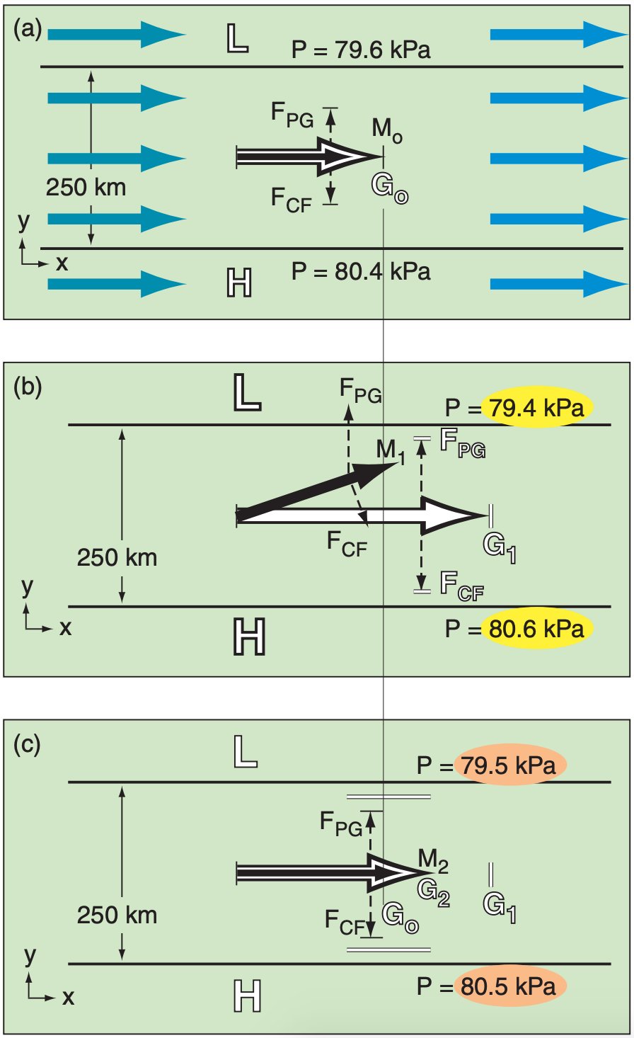
Picture a wind field (grey arrows in Fig. 11.19a) initially in geostrophic equilibrium (Mo = Go) at altitude 2 km above sea level (thus, no drag at ground). We will focus on just one of those arrows (the black arrow in the center), but all the wind vectors will march together, performing the same maneuvers.
Next, suppose an external process increases the horizontal pressure gradient to the value shown in Fig. 11.19b, with the associated faster theoretical geostrophic wind speed G1. Inertia prevents instantaneous response of the actual wind M. During this transition, pressure-gradient force FPG is greater than Coriolis force FCF. This force imbalance turns the wind M1 slightly toward low pressure and accelerates the air (Fig. 11.19b).
The component of wind M1 from high to low pressure horizontally moves air molecules, weakening the pressure field and thereby reducing the theoretical geostrophic wind (G2 in Fig. 11.19c). Namely, the wind field changed the mass (i.e., pressure) field. Simultaneously the actual wind accelerates to M2. Thus, the mass field also changed the wind field. After both fields have adjusted, the result is M2 > Mo and G2 < G1, with M2 = G2. These changes are called geostrophic adjustments.
Define a “disturbance” as the region that was initially forced out of equilibrium. As you move further away from the disturbance, the amount of geostrophic adjustment diminished. The e-folding distance for this reduction is
\(\ \begin{align} \lambda_{R}=\frac{N_{B V} \cdot Z_{T}}{f_{c}}\tag{11.12}\end{align}\)
where λR is known as the internal Rossby deformation radius. The Coriolis parameter is fc, tropospheric depth is ZT, and the Brunt-Väisälä frequency is NBV (see eq. on page 372). λR is roughly 1300 km.
For a given wavelength λ of the initial disturbance, eq. (11.12) can be used as follows. For large disturbances (λ > λR), the wind field experiences the greatest adjustment. For smaller λ, the pressure and temperature fields have the greatest adjustment.
Sample Application
Find the internal Rossby radius of deformation in a standard atmosphere at 45°N.
Find the Answer
Given: ϕ = 45°. Standard atmosphere from Chapter 1: T(z = ZT =11 km) = –56.5°C, T(z=0) = 15°C.
Find: λR = ? km
First, find fc = (1.458x10⁻⁴ s–1)·sin(45°) = 1.031x10⁻⁴ s–1
Next, find the average temperature and temperature difference across the depth of the troposphere:
Tavg = 0.5·(–56.5 + 15.0)°C = –20.8°C = 252 K
∆T = (–56.5 – 15.0) °C = –71.5°C across ∆z = 11 km
Find the Brunt-Väisälä frequency (see the Atmos. Stability chapter). \(N_{B V}=\sqrt{\frac{(9.8 \mathrm{m} / \mathrm{s})}{252 \mathrm{K}}\left[\frac{-71.5 \mathrm{K}}{11000 \mathrm{m}}+0.0098 \frac{\mathrm{K}}{\mathrm{m}}\right]}=0.0113 \mathrm{s}^{-1}\)
where the temperature differences in square brackets can be expressed in either °C or Kelvin.
Finally, use eq. (11.12): λR = (0.0113 s–1)·(11 km) / (1.031x10⁻⁴ s–1) = 1206 km
Check: Physics, units & magnitude are reasonable.
Exposition: When a cold-front over the Pacific approaches the steep mountains of western Canada, the front feels the influence of the mountains 1200 to 1300 km before reaching the coast, and begins to slow down.


