10.0: Winds and Weather Maps

10.1.1. Heights on Constant-Pressure Surfaces

Pressure-gradient force is the most important force because it is the only one that can drive winds in the horizontal. Other horizontal forces can alter an existing wind, but cannot create a wind from calm air. All the forces, including pressure-gradient force, are explained in the next sections. However, to understand the pressure gradient, we must first understand pressure and its atmospheric variation.

We can create weather maps showing values of the pressures measured at different horizontal locations all at the same altitude, such as at mean sea-level (MSL). Such a map is called a constant height map. However, one of the peculiarities of meteorology is that we can also create maps on other surfaces, such as on a surface connecting points of equal pressure. This is called an isobaric map. Both types of maps are used extensively in meteorology, so you should learn how they are related.

In Cartesian coordinates (x, y, z), z is height above some reference level, such as the ground or sea level. Sometimes we use geopotential height H in place of z, giving a coordinate set of (x, y, H) (see Chapter 1).

Can we use pressure as an alternative vertical coordinate instead of z? The answer is yes, because pressure changes monotonically with altitude. The word monotonic means that the value of the dependent variable changes in only one direction (never decreases, or never increases) as the value of the independent variable increases. Because P never increases with increasing z, it is indeed monotonic, allowing us to define pressure coordinates (x, y, P).

An isobaric surface is a conceptual curved surface that connects points of equal pressure, such as the shaded surface in Fig. 10.2b. The surface is higher above sea level in high-pressure regions, and lower in low-pressure regions. Hence the height contour lines for an isobaric surface are good surrogates for pressures lines (isobars) on a constant height map. Contours on an isobaric map are analogous to elevation contours on a topographic map; namely, the map itself is flat, but the contours indicate the height of the actual surface above sea level.

High pressures on a constant height map correspond to high heights of an isobaric map. Similarly, regions on a constant-height map that have tight packing (close spacing) of isobars correspond to regions on isobaric maps that have tight packing of height contours, both of which are regions of strong pressure gradients that can drive strong winds. This one-to-one correspondence of both types of maps (Figs. 10.2c & d) makes it easier for you to use them interchangeably.

Figure 10.2 Sketch of the similarity of (c) pressures drawn on a constant height surface to (d) heights drawn on a constant pressure surface. At any one height such as z = 5 km (shown by the thin dotted line in the vertical cross section of Fig. a), pressures at one location on the map might differ from pressure at other locations. In this example, a pressure of 50 kPa is located midway between the east and west limits of the domain at 5 km altitude. Pressure always decreases with increasing height z, as sketched in the vertical cross section of (a). Thus, at the other locations on the cross section, the 50 kPa pressure will be found at higher altitudes, as sketched by the thick dashed line. This thick dashed line and the corresponding thin dotted straight line are copied into the 3-D view of the same scenario is sketched in Fig. b. “L” indicates the cyclone center, having low pressure and low heights.

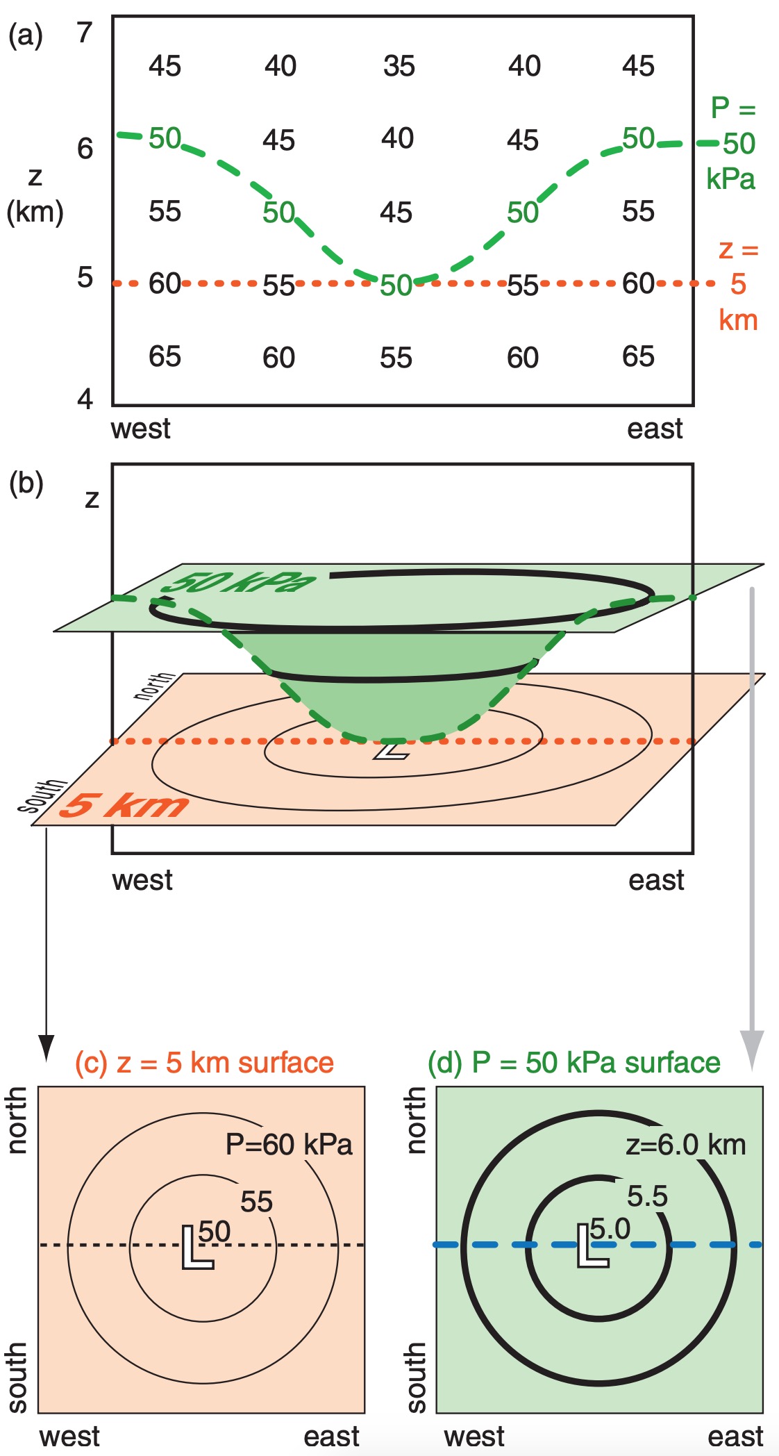
Isobaric surfaces can intersect the ground, but two different isobaric surfaces can never intersect because it is impossible to have two different pressures at the same point. Due to the smooth monotonic decrease of pressure with height, isobaric surfaces cannot have folds or creases.

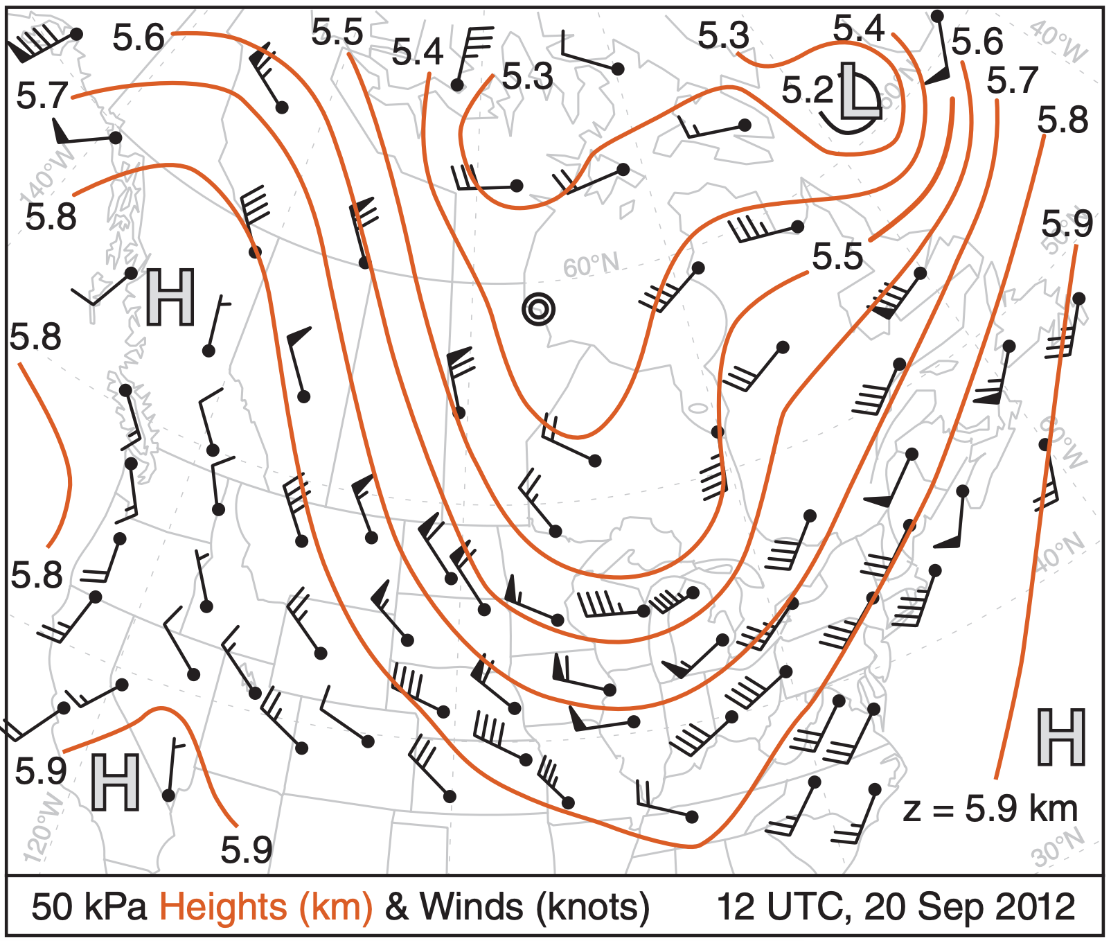
We will use isobaric charts for most of the upper-air weather maps in this book when describing upper-air features (mostly for historical reasons; see INFO box). Fig. 10.3 is a sample weather map showing height contours of the 50 kPa isobaric surface.

10.1.2. Plotting Winds

Symbols on weather maps are like musical notes in a score — they are a shorthand notation that concisely expresses information. For winds, the symbol is an arrow with feathers (or barbs and pennants). The tip of the arrow is plotted over the observation (weather-station) location, and the arrow shaft is aligned so that the arrow points toward where the wind is going. The number and size of the feathers indicates the wind speed (Table 10-1, copied from Table 9-9). Fig. 10.3 illustrates wind barbs.

Table 10-1. Interpretation of wind barbs.

Symbol	Wind Speed	Description
	calm	two concentric circles
	1 - 2 speed units	shaft with no barbs
	5 speed units	a half barb (half line)
	10 speed units	each full barb (full line)
	50 speed units	each pennant (triangle)
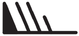The total speed is the sum of all barbs and pennants. For example, indicates a wind from the west at speed 75 units. Arrow tip is at the observation location. CAUTION: Different organizations use different speed units, such as knots, m s^–1, miles h^–1, km h^–1, etc. Look for a legend to explain the units. When in doubt, assume knots — the WMO standard. For unit conversion, a good approximation is 1 m s^–1 ≈ 2 knots.

Sample Application

Draw wind barb symbol for winds from the: (a) northwest at 115 knots; (b) northeast at 30 knots.

Find the Answer

(a) 115 knots = 2 pennants + 1 full barb + 1 half barb. (b) 30 knots = 3 full barbs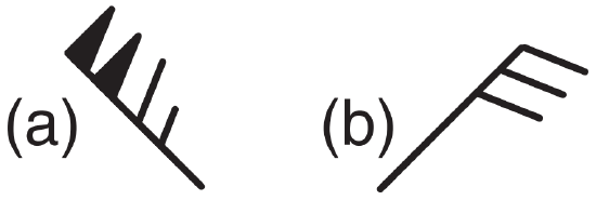

Check: Consistent with Table 10-1.

Exposition: Feathers (barbs & pennants) should be on the side of the shaft that would be towards low pressure if the wind were geostrophic.

INFO • Why use isobaric maps?

There are five reasons for using isobaric charts.

1. During the last century, the radiosonde (a weather sensor hanging from a free helium balloon that rises into the upper troposphere and lower stratosphere) could not measure its geometric height, so instead it reported temperature and humidity as a function of pressure. For this reason, upper-air charts (i.e., maps showing weather above the ground) traditionally have been drawn on isobaric maps.
2. Aircraft altimeters are really pressure gauges. Aircraft assigned by air-traffic control to a specific “altitude” above 18,000 feet MSL will actually fly along an isobaric surface. Many weather observations and forecasts are motivated by aviation needs.
3. Air pressure is created by the weight of air molecules. Thus, every point on an isobaric map has the same mass of air molecules above it.
4. An advantage of using equations of motion in pressure coordinates is that you do not need to consider density, which is not routinely observed.
5. Some numerical weather prediction models use reference pressures that vary hydrostatically with altitude.

Items (1) and (5) are less important these days, because modern radiosondes use GPS (Global Posi- tioning System) to determine their (x, y, z) position. So they report all meteorological variables (including pressure) as a function of z. Also, some of the modern weather forecast models do not use pressure as the vertical coordinate. Perhaps future weather analyses and numerical predictions will be shown on constant-height maps.

Figure 10.3 Winds (1 knot ≈ 0.5 m s^–1) and heights (km) on the 50 kPa isobaric surface. The relative maxima and minima are labeled as H (high heights) and L (low heights). Table 10-1 explains winds.