
5.7: An Air Parcel and its Environment
- Page ID
- 9559

\( \newcommand{\vecs}[1]{\overset { \scriptstyle \rightharpoonup} {\mathbf{#1}} } \)
\( \newcommand{\vecd}[1]{\overset{-\!-\!\rightharpoonup}{\vphantom{a}\smash {#1}}} \)
\( \newcommand{\dsum}{\displaystyle\sum\limits} \)
\( \newcommand{\dint}{\displaystyle\int\limits} \)
\( \newcommand{\dlim}{\displaystyle\lim\limits} \)
\( \newcommand{\id}{\mathrm{id}}\) \( \newcommand{\Span}{\mathrm{span}}\)
( \newcommand{\kernel}{\mathrm{null}\,}\) \( \newcommand{\range}{\mathrm{range}\,}\)
\( \newcommand{\RealPart}{\mathrm{Re}}\) \( \newcommand{\ImaginaryPart}{\mathrm{Im}}\)
\( \newcommand{\Argument}{\mathrm{Arg}}\) \( \newcommand{\norm}[1]{\| #1 \|}\)
\( \newcommand{\inner}[2]{\langle #1, #2 \rangle}\)
\( \newcommand{\Span}{\mathrm{span}}\)
\( \newcommand{\id}{\mathrm{id}}\)
\( \newcommand{\Span}{\mathrm{span}}\)
\( \newcommand{\kernel}{\mathrm{null}\,}\)
\( \newcommand{\range}{\mathrm{range}\,}\)
\( \newcommand{\RealPart}{\mathrm{Re}}\)
\( \newcommand{\ImaginaryPart}{\mathrm{Im}}\)
\( \newcommand{\Argument}{\mathrm{Arg}}\)
\( \newcommand{\norm}[1]{\| #1 \|}\)
\( \newcommand{\inner}[2]{\langle #1, #2 \rangle}\)
\( \newcommand{\Span}{\mathrm{span}}\) \( \newcommand{\AA}{\unicode[.8,0]{x212B}}\)
\( \newcommand{\vectorA}[1]{\vec{#1}} % arrow\)
\( \newcommand{\vectorAt}[1]{\vec{\text{#1}}} % arrow\)
\( \newcommand{\vectorB}[1]{\overset { \scriptstyle \rightharpoonup} {\mathbf{#1}} } \)
\( \newcommand{\vectorC}[1]{\textbf{#1}} \)
\( \newcommand{\vectorD}[1]{\overrightarrow{#1}} \)
\( \newcommand{\vectorDt}[1]{\overrightarrow{\text{#1}}} \)
\( \newcommand{\vectE}[1]{\overset{-\!-\!\rightharpoonup}{\vphantom{a}\smash{\mathbf {#1}}}} \)
\( \newcommand{\vecs}[1]{\overset { \scriptstyle \rightharpoonup} {\mathbf{#1}} } \)
\(\newcommand{\longvect}{\overrightarrow}\)
\( \newcommand{\vecd}[1]{\overset{-\!-\!\rightharpoonup}{\vphantom{a}\smash {#1}}} \)
\(\newcommand{\avec}{\mathbf a}\) \(\newcommand{\bvec}{\mathbf b}\) \(\newcommand{\cvec}{\mathbf c}\) \(\newcommand{\dvec}{\mathbf d}\) \(\newcommand{\dtil}{\widetilde{\mathbf d}}\) \(\newcommand{\evec}{\mathbf e}\) \(\newcommand{\fvec}{\mathbf f}\) \(\newcommand{\nvec}{\mathbf n}\) \(\newcommand{\pvec}{\mathbf p}\) \(\newcommand{\qvec}{\mathbf q}\) \(\newcommand{\svec}{\mathbf s}\) \(\newcommand{\tvec}{\mathbf t}\) \(\newcommand{\uvec}{\mathbf u}\) \(\newcommand{\vvec}{\mathbf v}\) \(\newcommand{\wvec}{\mathbf w}\) \(\newcommand{\xvec}{\mathbf x}\) \(\newcommand{\yvec}{\mathbf y}\) \(\newcommand{\zvec}{\mathbf z}\) \(\newcommand{\rvec}{\mathbf r}\) \(\newcommand{\mvec}{\mathbf m}\) \(\newcommand{\zerovec}{\mathbf 0}\) \(\newcommand{\onevec}{\mathbf 1}\) \(\newcommand{\real}{\mathbb R}\) \(\newcommand{\twovec}[2]{\left[\begin{array}{r}#1 \\ #2 \end{array}\right]}\) \(\newcommand{\ctwovec}[2]{\left[\begin{array}{c}#1 \\ #2 \end{array}\right]}\) \(\newcommand{\threevec}[3]{\left[\begin{array}{r}#1 \\ #2 \\ #3 \end{array}\right]}\) \(\newcommand{\cthreevec}[3]{\left[\begin{array}{c}#1 \\ #2 \\ #3 \end{array}\right]}\) \(\newcommand{\fourvec}[4]{\left[\begin{array}{r}#1 \\ #2 \\ #3 \\ #4 \end{array}\right]}\) \(\newcommand{\cfourvec}[4]{\left[\begin{array}{c}#1 \\ #2 \\ #3 \\ #4 \end{array}\right]}\) \(\newcommand{\fivevec}[5]{\left[\begin{array}{r}#1 \\ #2 \\ #3 \\ #4 \\ #5 \\ \end{array}\right]}\) \(\newcommand{\cfivevec}[5]{\left[\begin{array}{c}#1 \\ #2 \\ #3 \\ #4 \\ #5 \\ \end{array}\right]}\) \(\newcommand{\mattwo}[4]{\left[\begin{array}{rr}#1 \amp #2 \\ #3 \amp #4 \\ \end{array}\right]}\) \(\newcommand{\laspan}[1]{\text{Span}\{#1\}}\) \(\newcommand{\bcal}{\cal B}\) \(\newcommand{\ccal}{\cal C}\) \(\newcommand{\scal}{\cal S}\) \(\newcommand{\wcal}{\cal W}\) \(\newcommand{\ecal}{\cal E}\) \(\newcommand{\coords}[2]{\left\{#1\right\}_{#2}}\) \(\newcommand{\gray}[1]{\color{gray}{#1}}\) \(\newcommand{\lgray}[1]{\color{lightgray}{#1}}\) \(\newcommand{\rank}{\operatorname{rank}}\) \(\newcommand{\row}{\text{Row}}\) \(\newcommand{\col}{\text{Col}}\) \(\renewcommand{\row}{\text{Row}}\) \(\newcommand{\nul}{\text{Nul}}\) \(\newcommand{\var}{\text{Var}}\) \(\newcommand{\corr}{\text{corr}}\) \(\newcommand{\len}[1]{\left|#1\right|}\) \(\newcommand{\bbar}{\overline{\bvec}}\) \(\newcommand{\bhat}{\widehat{\bvec}}\) \(\newcommand{\bperp}{\bvec^\perp}\) \(\newcommand{\xhat}{\widehat{\xvec}}\) \(\newcommand{\vhat}{\widehat{\vvec}}\) \(\newcommand{\uhat}{\widehat{\uvec}}\) \(\newcommand{\what}{\widehat{\wvec}}\) \(\newcommand{\Sighat}{\widehat{\Sigma}}\) \(\newcommand{\lt}{<}\) \(\newcommand{\gt}{>}\) \(\newcommand{\amp}{&}\) \(\definecolor{fillinmathshade}{gray}{0.9}\)Consider the column of air that is fixed (Eulerian framework) over any small area on the globe. Let this air column represent a stationary environment through which other things (aircraft, raindrops, air parcels) can move.
For an air parcel that moves through this environment, we can follow the parcel (Lagrangian framework) to determine how its thermodynamic state might change as it moves to different altitudes. As a first approximation, we often assume that there is no mixing between the air parcel and the surrounding environment.
5.6.1. Soundings
As stated at the start of this chapter, the vertical profile of environmental conditions is called an upper-air sounding, or just a sounding. The word “sounding” is used many ways. It is the:
- activity of collecting the environment data (as in “to make a sounding”).
- data that was so collected (as in “to analyze the sounding data”).
- resulting plot of these data on a thermo diagram (as in “the sounding shows a deep unstable layer”).
A sonde is an expendable weather instrument with built-in radio transmitter that can be attached to a platform that moves up or down through the air column to measure its environmental state. Helium-filled latex weather balloons carry radiosondes to measure thermodynamic state (P, T, Td) or carry rawinsondes measure (z, P, T, Td, U, V) by also utilizing GPS or other navigation signals. Rocketsondes are lofted by small sounding rockets, and dropsondes are dropped by parachute from aircraft. Unmanned aerial vehicles (UAVs, drones) and conventional aircraft can carry weather sensors. Radar and satellites are remote sensors that can also measure portions of soundings.
The sounding represents a snapshot of the state of the air in the environment, such as in the Sample Application on this page. The plot of any dependent variable vs. height or pressure is called a vertical profile. The negative of the vertical temperature gradient (–∆Te /∆z) is defined as the environmental lapse rate, where subscript e means environment.
Normally, temperature and dew point are plotted at each height. Other chemicals such as smoke particles or ozone can also be plotted as a sounding. It is difficult to measure density, so instead its value at any height is calculated from the ideal gas law. For cloudy air, the Td points coincide with the T points. Most sondes have some imprecision, so we infer clouds in any layer where Td is near T.
Straight lines are drawn connecting the temperature points (see INFO box on mandatory and significant levels), and separate straight lines are drawn for the humidity points for unsaturated air. Liquid or ice mixing ratios are not usually measured by radiosondes, but can be obtained by research aircraft flying slant ascent or descent soundings.
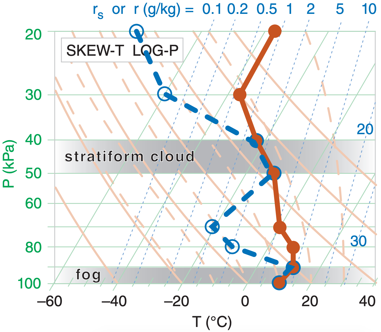
Sample Application
Plot the following data on a skew-T log-P diagram.
| P (kPa) | T (°C) | Td (°C) |
| 20 | –36 | –80 |
| 30 | –36 | –60 |
| 40 | –23 | –23 |
| 50 | –12 | –12 |
| 70 | 0 | –20 |
| 80 | 8 | –10 |
| 90 | 10 | 10 |
| 100 | 10 | 10 |
Find the Answer
Here I used red for temperature (T) and blue for dewpoint (Td). Always connect the data points with straight lines.
Check: Sketches OK. Also, dew point is never greater than temperature, as required.
Exposition: There are two levels where dew-point temperature equals the actual air temperature, and these two levels correspond to saturated (cloudy) air. The bottom layer is fog, and the elevated one would be a mid-level stratiform (layered) cloud. In the Clouds chapter you will learn that this type of mid-altitude cloud is called altostratus or altocumulus.
There are also two layers of dry air, where there is a large spread between T and Td. These layers are roughly 80 to 60 kPa, and 35 to 20 kPa.
Rising rawinsondes record the weather at ∆z ≈ 5 m increments, yielding data at about 5000 heights. To reduce the amount of data transmitted to weather centers, straight-line segments are fit to the sounding, and only the end points of the line segments are reported. These points, called significant levels, are at the kinks in the sounding (as plotted in the previous Sample Application). Additional mandatory levels at the surface and 100, 92.5, 85, 70, 50, 40, 30, 25, 20, 15, 10, 7, 5, 3, 2, & 1 kPa are also reported, to make it easier to analyze upper-air charts at these levels.
5.6.2. Buoyant Force
For an object such as an air parcel that is totally immersed in a fluid (air), buoyant force per unit mass (F/m) depends on the density difference between the object (ρo) and the surrounding fluid (ρf ):
\(\ \begin{align} \dfrac{F}{m}=\dfrac{\rho_{o}-\rho_{f}}{\rho_{o}} \cdot g=g^{\prime}\tag{5.2}\end{align}\)
where gravitational acceleration (negative downward) is g = –9.8 m·s–2. If the immersed object is positively buoyant (F = positive) then the buoyant force pulls upward. Negatively buoyant objects (F = negative) are pulled downward, while neutrally buoyant objects have zero buoyant force.
Recall that weight is the force caused by gravity acting on a mass (F = m·g). Since buoyancy changes the net force (makes the weight less), the net effect on the object is that of a reduced gravity (g’) as defined in eq. (5.2). Thus F = m·g’.
Identify the air parcel (subscript p) as the object, and the environment (subscript e) as the surrounding fluid. Because both air parcels and the surrounding environment are made of air, use the ideal gas law (P = ρ ℜ Tv) to describe the densities in eq. (5.2).
\(\ \begin{align} \dfrac{F}{m}=\dfrac{T_{v e}-T_{v p}}{T_{v e}} \cdot g=g^{\prime}\tag{5.3a}\end{align}\)
where the pressure inside the parcel is assumed to always equal that of the surrounding environment at the same height, allowing the pressures from the ideal gas law to cancel each other in eq. (5.3a).
Virtual temperature Tv (in Kelvins) is used to account for the effects of both temperature and water vapor on the buoyancy. For relatively dry air, Tv ≈ T, giving:
\(\ \begin{align} \dfrac{F}{m} \approx \dfrac{T_{p}-T_{e}}{T_{e}} \cdot|g|=g^{\prime}\tag{5.3b}\end{align}\)
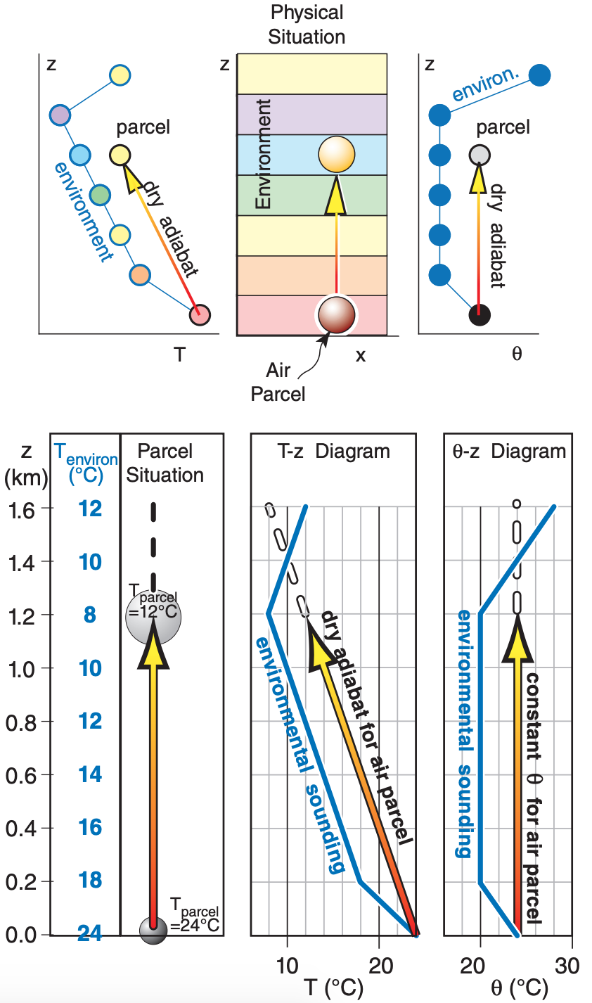
Namely, parcels warmer than their environment tend to rise. Colder parcels tend to sink. As air parcels move vertically, their temperatures change as given by adiabatic (dry or saturated) lapse rates, so you need to repeatedly re-evaluate the buoyancy of the parcel relative to its new local environment. Thermo diagrams are extremely handy for this, as sketched in Figure 5.12.
Sample Application
When the air parcel in Figure 5.12 reaches 1 km altitude, what is its buoyant force/mass? The air is dry.
Find the Answer
Given: Te = 10°C +273 = 283 K, Tp = 14°C +273 = 287 K
Find: F/m = ? m·s–2
Apply eq. (5.3a) for dry air:
F/m = (287 K – 283 K)·(9.8 m·s–2) / 283 K
= 0.14 m·s–2 = 0.14 N/kg (see units in Appendix A)
Check: Physics and units are reasonable.
Exposition: Positive buoyancy force favors rising air.
Sometimes it is more convenient to use virtual potential temperature θv (eqs. 3.13, 3.14) to calculate buoyant force, because adiabatic parcel motion has constant θv p. Buoyant force per mass is then:
\(\ \begin{align} \dfrac{F}{m}=\dfrac{\theta_{v e}-\theta_{v p}}{T_{v e}} \cdot g=g^{\prime}\tag{5.3c}\end{align}\)
where gravitational acceleration (g = –9.8 m s–2) is a negative number in eq. (5.3c) because it acts downward. Subscript e indicates “environment”.
Many meteorologists prefer to use the magnitude of gravitational acceleration as a positive number:
\(\ \begin{align} \dfrac{F}{m}=\dfrac{\theta_{v p}-\theta_{v e}}{T_{v e}} \cdot|g|=g^{\prime}\tag{5.3d}\end{align}\)
which more obviously shows that upward buoyancy force occurs for a parcel warmer than the environment at its same altitude or pressure.
Picture the physical situation in the left third of Figure 5.12 on the previous page. Suppose you grab a small piece of the environmental air near the ground and lift it. As the parcel rises, it cools adiabatically. It is moving through a somewhat static environment, and thus is encountering different surrounding (environmental) temperatures at different altitudes (represented by the colored background). Namely, both the parcel temperature and the environmental temperature are different at different altitudes.
We need to know these different temperatures at each altitude in order to determine the temperature difference and the resulting parcel buoyancy from eqs. (5.3). To make our lives easier, we use thermo diagrams on which we can plot the background environment, and which show dry adiabats as relate to parcel rise. Two examples are the emagram and θ-Z diagrams in Figure 5.12. These both represent the same parcel and same environment.
Sample Application
a) Use a thermo diagram to estimate the potentialtemperature values for each point in the environmental sounding, and plot your answers a new, linear graph of θ vs. P. Assume dry air. Environmental sounding: [P(kPa), T(°C)] = [100, 20], [95, 10], [85, 0], [75, 0], [70, –4]
b) An air parcel at [P(kPa), T(°C)] = [100, 23] moves to a new height of 80 kPa. Plot its path on your θ vs. P graph, and find its new buoyant force/mass at 80 kPa.
Find the Answer
Given: The T vs. P data above. Dry, thus Tv = T.
Find: (a) Estimate θ from thermo diag. & plot vs. P.
(b) Plot parcel rise on the same graph.
Calculate buoyant F/m at P = 80 kPa.
Method
a) From the large thermo diagrams at the chapter end, the environment potential temperature sounding is: [P(kPa), θ(°C)], [100,20], [95,15], [85,15], [75,25], [70,26]
See blue line in the figure:
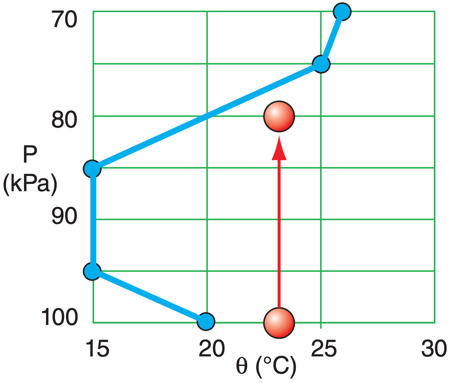
b) The parcel initial state is [P(kPa), θ(°C)] = [100,23]. See red line in figure. At P = 80 kPa, the figure shows ∆θ = 23 – 20°C = 3°C = 3 K. Because dry air: ∆θv = ∆θ. Tv = T ≈ 10°C = 283 K as approximate average T.
Apply eq. (5.3d):
F/m = (3K/283K)·(9.8 m s–2) = 0.10 m s–2 = 0.10 N kg–1
Check: Physics and units are reasonable.
Exposition: The upward buoyancy force causes the air parcel to continue to rise, until it hits the blue line.
5.6.3. Brunt-Väisälä Frequency
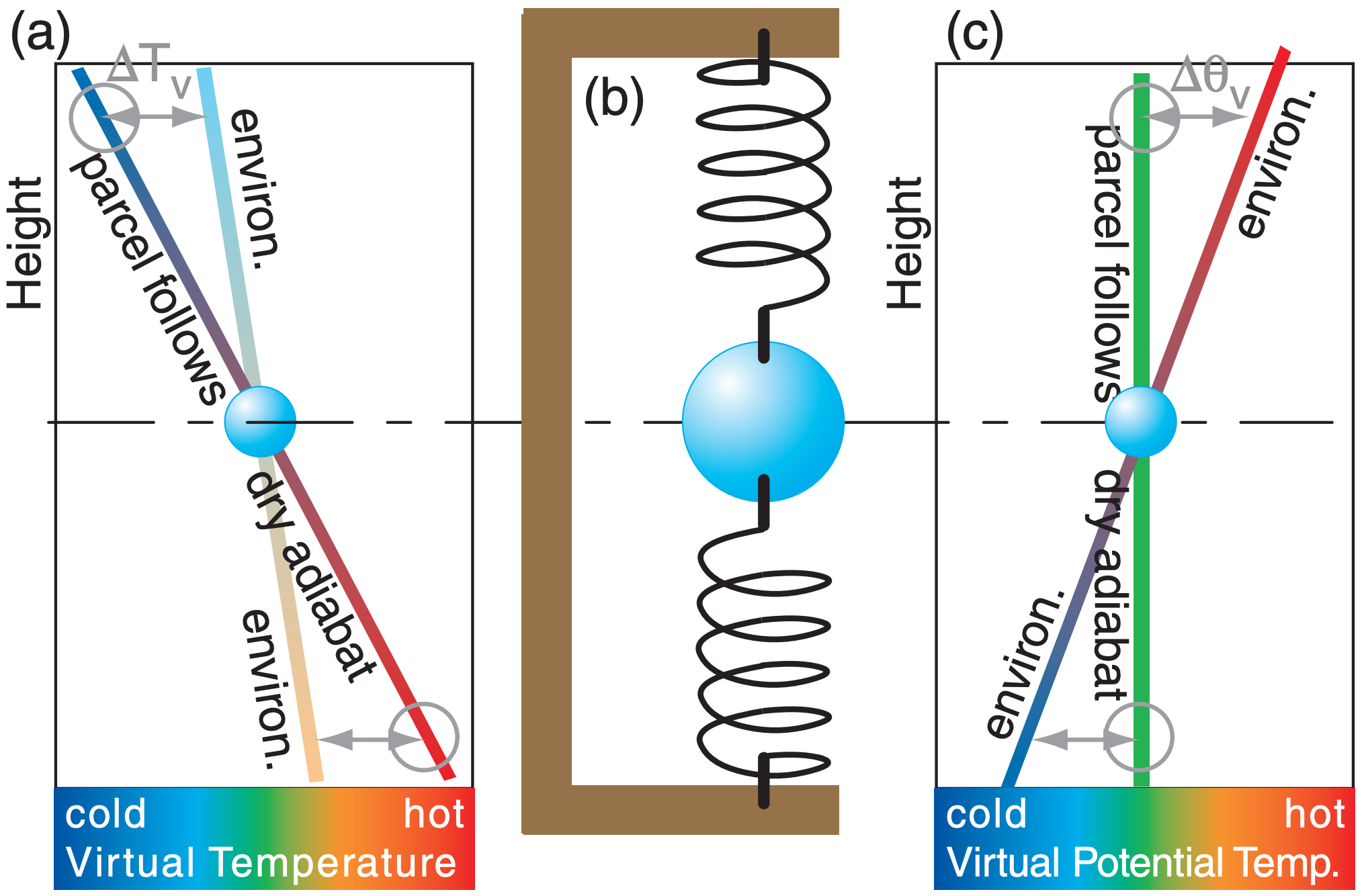
Suppose the ambient environment lapse rate Γ is less than the dry adiabatic lapse rate (Γd = 9.8°C km–1). Namely, temperature does not decrease as fast with increasing height as Γd (see Figure 5.13a).
Suppose you start with an air parcel having the same initial temperature as the environment (the blue sphere in Figure 5.13a) at any initial altitude. If you push the air parcel down, it warms at the adiabatic lapse rate, which makes it warmer than the surrounding environment at its new height. This positive buoyant force would tend to push the parcel upward. The parcel’s inertia would cause it to overshoot upward past its initial height, where adiabatic cooling would create a negative buoyant force that reverses the parcel’s upward motion.
In summary, a parcel that is displaced vertically from its initial altitude will oscillate up and down. The environment that enables such an oscillation is said to be statically stable. The oscillation is similar to that experienced by a vertically displaced weight suspended between two elastic bands (Figure 5.13b).
The air parcel oscillates vertically with frequency (radians s–1)
\(\ \begin{align} N_{B V}=\sqrt{\dfrac{|g|}{T_{v}} \cdot\left(\dfrac{\Delta T_{v}}{\Delta z}+\Gamma_{d}\right)}\tag{5.4a}\end{align}\)
where NBV is the Brunt-Väisälä frequency, and |g| = 9.8 m s–2 is the magnitude of gravitational acceleration. Virtual temperature Tv must be used to account for water vapor, which has lower density than dry air. If the air is relatively dry, then Tv ≈ T. Use absolute units (K) for Tv in the denominator.
The same frequency can be expressed in terms of virtual potential temperature θv (see Figure 5.13c):
\(\ \begin{align} N_{B V}=\sqrt{\dfrac{|g|}{T_{v}} \cdot \dfrac{\Delta \theta_{v}}{\Delta z}}\tag{5.4b}\end{align}\)
The oscillation period is
\(\ \begin{align} P_{B V}=\dfrac{2 \pi}{N_{B V}}\tag{5.5}\end{align}\)
If the static stability weakens (as the environmental ∆T/∆z approaches –Γd), then the frequency decreases and the period increases toward infinity. The equations above are idealized, and neglect the damping of the oscillation due to air drag (friction).
Sample Application
For a dry standard-atmosphere defined in Chapter 1, find the Brunt-Väisälä frequency & period at z = 4 km.
Find the Answer
Given: ∆T/∆z = –6.5 K/km from eq. (1.16).
Tv = T because dry air.
Use Table 1-5 at z = 4 km to get: T = –11°C = 262 K Find: NBV = ? rad s–1, PBV = ? s
Apply eq. (5.4a)
\(N_{B V}=\sqrt{\dfrac{\left(9.8 \mathrm{ms}^{-2}\right)}{262 \mathrm{K}} \cdot\left(-6.5+9.8 \dfrac{\mathrm{K}}{\mathrm{km}}\right) \cdot\left(\dfrac{1 \mathrm{km}}{1000 \mathrm{m}}\right)}\)
= [ 1.234x10⁻⁴ s–2] 1/2 = 0.0111 rad s–1
Apply eq. (5.5):
\(P_{B V}=\dfrac{2 \pi \text { radians }}{0.0111 \text { radians } / \mathrm{s}}=565.5 \mathrm{s}=9.4 \mathrm{min}\)
Check: Physics and units are reasonable.
Exposition: The Higher Math box at right shows that NBV must have units of (radians s–1) because it is the argument of a sine function. But meteorologists often write the units as (s–1), where the radians are implied.
Create the Governing Equations
Consider a scenario as sketched in Figure 5.13a, where the environment lapse rate is Γ and the dry adiabatic lapse rate is Γd. Define the origin of a coordinate system to be where the two lines cross in that figure, and let z be height above that origin. Consider dry air for simplicity (Tv = T). Based on geometry, Figure 5.13a shows that the temperature difference between the two lines at height z is ∆T = (Γ – Γd)·z.
Eq. (5.3b) gives the corresponding vertical force F per unit mass m of the air parcel:
F/m = |g|·∆T/Te = |g|·[(Γ – Γd)·z]/Te
But F/m = a according to Newton’s 2nd law, where acceleration a ≡ d2z/dt2. Combining these eqs. gives:
\(\dfrac{\mathrm{d}^{2} z}{\mathrm{d} t^{2}}=\dfrac{|g|}{T_{e}} \cdot\left(\Gamma-\Gamma_{d}\right) \cdot z\)
Because Te is in Kelvin, it varies by only a small percentage as the air parcel oscillates, so approximate it with the average environmental temperature \(\ \bar{T_e}\) over the vertical span of oscillation.
All factors on the right side of the eq. above are constant except for z, so to simplify the notation, use a new variable NBV2 ≡ –|g|·(Γ – Γd)/ \(\ \bar{T_e}\) to represent those constant factors. [This definition agrees with eq. (5.4a) when you recall that Γ = –∆T/∆z .]
This leaves us with a second-order differential equation (a hyperbolic differential eq.) known as the wave equation:
\(\ \begin{align} \dfrac{\mathrm{d}^{2} z}{\mathrm{d} t^{2}}=-N_{B V}^{2} \cdot z\tag{5a}\end{align}\)
Solve the Differential Equation
For the wave equation, try a wave solution:
\(\ \begin{align} z=A \cdot \sin (f \cdot t)\tag{5b}\end{align}\)
with unknown amplitude A and unknown frequency of oscillation f (radians s–1). Insert (5b) in (5a) to get:
\(-f^{2} \cdot A \cdot \sin (f \cdot t)=-N_{B V}^{2} \cdot A \cdot \sin (f \cdot t)\)
After you cancel the A·sin(f·t) from each side, you get:
\(\ f=N_{B V}\)
Using this in eq. (5b) gives an air parcel height that oscillates in time:
\(\ \begin{align} z=A \cdot \sin \left(N_{B V} \cdot t\right)\tag{5c}\end{align}\)
Exposition
The amplitude A is the initial distance that you displace the air parcel from the origin. If you plug eq. (5.5) into (5c) you get: z = A·sin(2π·t/PBV), which gives one full oscillation during a time period of t = PBV.