
5.8: Flow Stability
- Page ID
- 9921

Stability is a characteristic of how a system reacts to small disturbances. If the disturbance is damped, the system is said to be stable. If the disturbance causes an amplifying response (irregular motions or regular oscillations), the system is unstable.
For fluid-flow stability we will focus on turbulent responses spanning the smallest eddies to deep thunderstorms. The stability characteristics are:
- Unstable air becomes, or is, turbulent (irregular, gusty, stormy).
- Stable air becomes, or is, laminar (non-turbulent, smooth, non-stormy).
- Neutral air has no tendency to change (disturbances neither amplify or dampen).
Flow stability is controlled by ALL the processes (buoyancy, inertia, wind shear, rotation, etc.) acting on the flow. However, to simplify our understanding of flow, we sometimes focus on just a subset of processes. If you ignore all processes except buoyancy, then you are studying static stability. If you include buoyancy and wind-shear processes, then you are studying dynamic stability.
5.7.1. Static Stability
One way to estimate static stability is by taking a small piece of the environment and hypothetically displacing it as an air parcel a small distance vertically from its starting point, assuming the surrounding environment is horizontally large and is quasi-stationary. Another is to lift whole environmental layers. We will look at both methods.
5.7.1.1. Parcel Method for Static Stability
Will a displaced air parcel experience buoyancy forces that push it in the same direction it was displaced (i.e., an amplifying or unstable response), or will buoyancy forces tend to push the parcel back to its starting (equilibrium) height (a stable response)?
The answer to this question is tricky, because the region of unstable response can span large vertical regions. For example, a parcel that is warmer than its environment will keep rising over large distances so long as it remains warmer than its surrounding environment at the same altitude as the parcel.
This type of buoyancy motion, called convection, stirs the air and generates turbulence over the whole span of its rise. Namely, a thin region that is locally stable might become turbulent if an air parcel moves through it from some distant source. Such distant effects are known as nonlocal turbulence, and must be considered when determining stability.
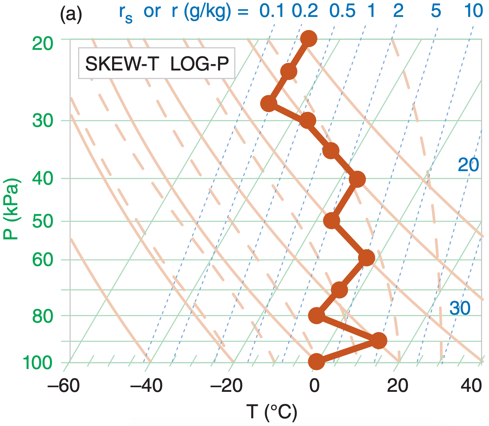
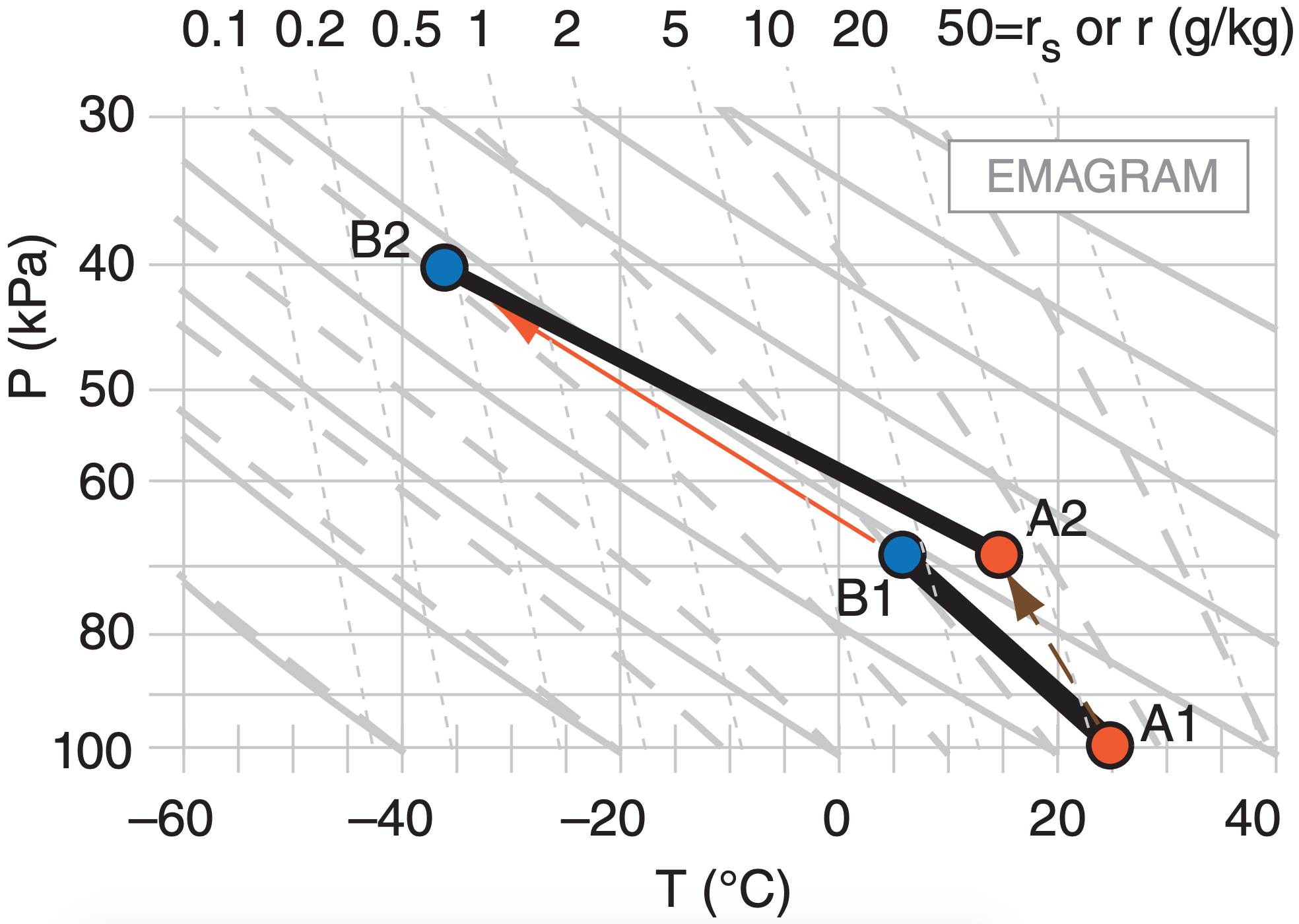
Step 1: Graphical methods are usually best for determining static stability, in order to account for nonlocal effects. Plot the environmental sounding on a thermo diagram (Figure 5.14a). Any type of thermo diagram will work — they all will give the same stability determination.
Step 2: At every apex (kink in the sounding), hypothetically displace an air parcel from that kink a small distance upward. If the parcel is unsaturated, follow a dry adiabat upward to determine the parcel’s new temperature. If saturated, follow a moist adiabat. If that displaced parcel experiences an upward buoyant force (i.e., is warmer than its surrounding environment at its displaced height), then it is locally unstable, so write the letter “U” just above that apex (Fig 5.14b). If the upward displaced parcel experiences no force (i.e., is nearly the same temperature as the environment at its displaced height), then write “N” just above that apex because it is locally neutral. If the upward displaced parcel experiences a downward force (i.e., is cooler than the environment at its displaced height), then write “S” just above the apex because it is locally stable.

Step 3: Do a similar exercise at every apex, but hypothetically displacing the air parcel downward (Figure 5.14c). If the parcel is cooler than its environment at its displaced height and experiences a downward force, then it is locally unstable, so write “U” just below that apex. If the parcel is the same temperature as the environment at its displaced height, write “N” just below the apex. If the parcel is warmer than the environment at its displaced height, then write “S” just below the apex.
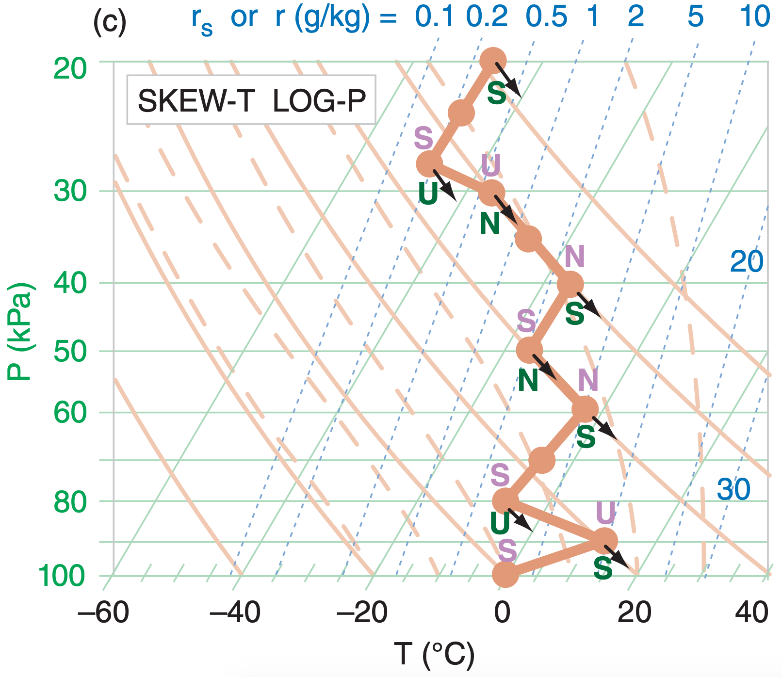
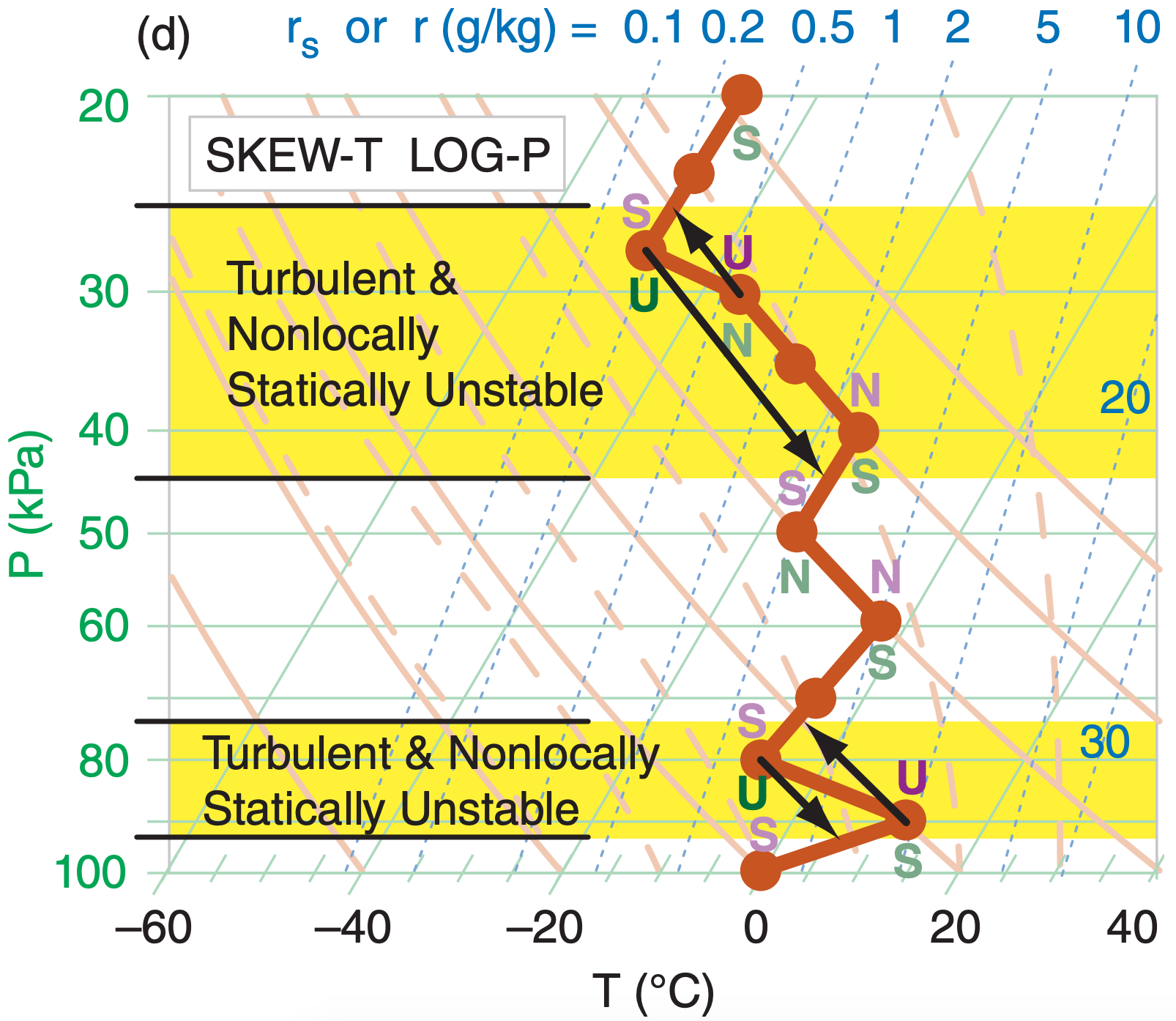
Step 4: From every apex with U above, draw an arrow that follows the adiabat upward until it hits the sounding (Figure 5.14d). From every apex with U below, draw an arrow that follows the adiabat downward until it hits the sounding. All domains spanned by these “U” arrows are turbulent and are nonlocally statically unstable. Any vertically overlapping “U” regions should be interpreted as one contiguous nonlocally unstable and turbulent region.
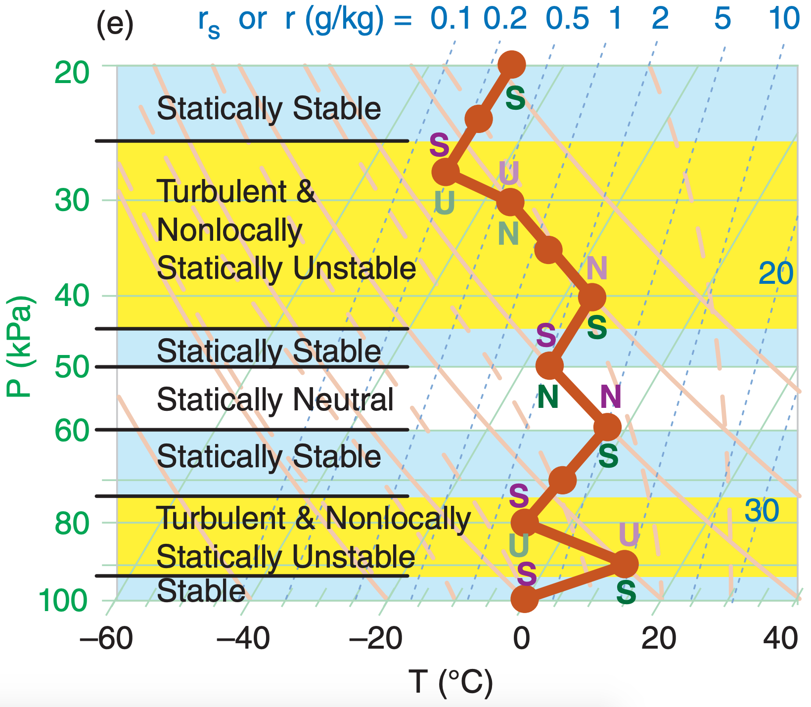
Step 5: Any regions outside of the unstable regions from the previous step are stable or neutral, as indicated by the “S” or “N” letters next to those sounding line segments (Figure 5.14e).
Within statically neutral subdomains, the vertical gradients of temperature T or potential temperature θ are:
\(\ \begin{align} \frac{\Delta T}{\Delta z} \approx-\left\{\begin{array}{ll}{\Gamma_{d}} & {\text { if unsaturated }} \\ {\Gamma_{s}} & {\text { if saturated }}\end{array}\right.\tag{5.6a}\end{align}\)
or
\(\ \begin{align} \frac{\Delta \theta}{\Delta z} \approx\left\{\begin{array}{ll}{0} & {\text { if unsaturated }} \\ {\Gamma_{d}-\Gamma_{s}} & {\text { if saturated }}\end{array}\right.\tag{5.6b}\end{align}\)
where Γd = 9.8 K km–1 is the dry adiabatic lapse rate, and Γs is the saturated (or moist) adiabatic lapse rate (which varies, but is always a positive number).
In statically stable subdomains, the temperature does not decrease with height as fast as the adiabatic rate (including isothermal layers, and temperature inversion layers where temperature increases with height). Thus:
\(\ \begin{align} \frac{\Delta T}{\Delta z}>-\left\{\begin{array}{ll}{\Gamma_{d}} & {\text { if unsaturated }} \\ {\Gamma_{s}} & {\text { if saturated }}\end{array}\right.\tag{5.7a}\end{align}\)
or
\(\ \begin{align} \frac{\Delta \theta}{\Delta z}>\left\{\begin{array}{ll}{0} & {\text { if unsaturated }} \\ {\Gamma_{d}-\Gamma_{s}} & {\text { if saturated }}\end{array}\right.\tag{5.7b}\end{align}\)
5.7.1.2. Layer Method for Static Stability
Sometimes a whole layer of environmental air is lifted or lowered by an outside process. Synoptic-scale warm and cold fronts (see the Fronts & Airmasses chapter) and coherent clusters of thunderstorms (mesoscale convective complexes, see the Thunderstorm chapters) are examples of layer-lifting processes. In these cases we cannot use the parcel method to determine static stability, because it assumes a quasi-stationary environment.
Lapse Rate Names
The lapse rate γ of an environmental layer is defined as the temperature decrease with height:
\(\ \begin{align} \gamma=-\Delta T / \Delta z\tag{5.8}\end{align}\)
Lapse rates are named as shown in Table 5-1, where isothermal and inversion are both subadiabatic.
| Table 5-1. Names of environmental lapse rates, where Γd is the dry adiabatic lapse rate. | ||
| Name | Layer Lapse Rate | Figure |
|---|---|---|
| adiabatic | γ = Γd = 9.8°C km–1 | 5.15(4) |
| superadiabatic | γ > Γd | 5.15(5) |
| subadiabatic | γ < Γd | 5.15(1) |
|
T = constant with z |
|
| • inversion | T = increases with z | |
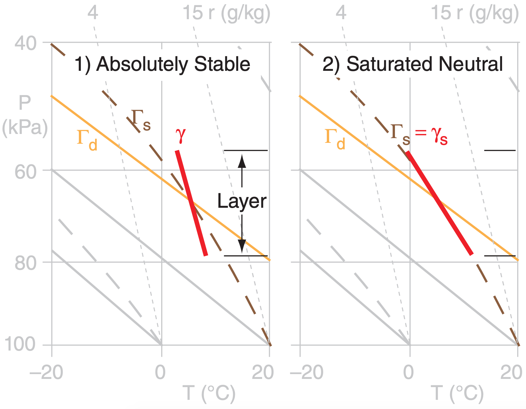
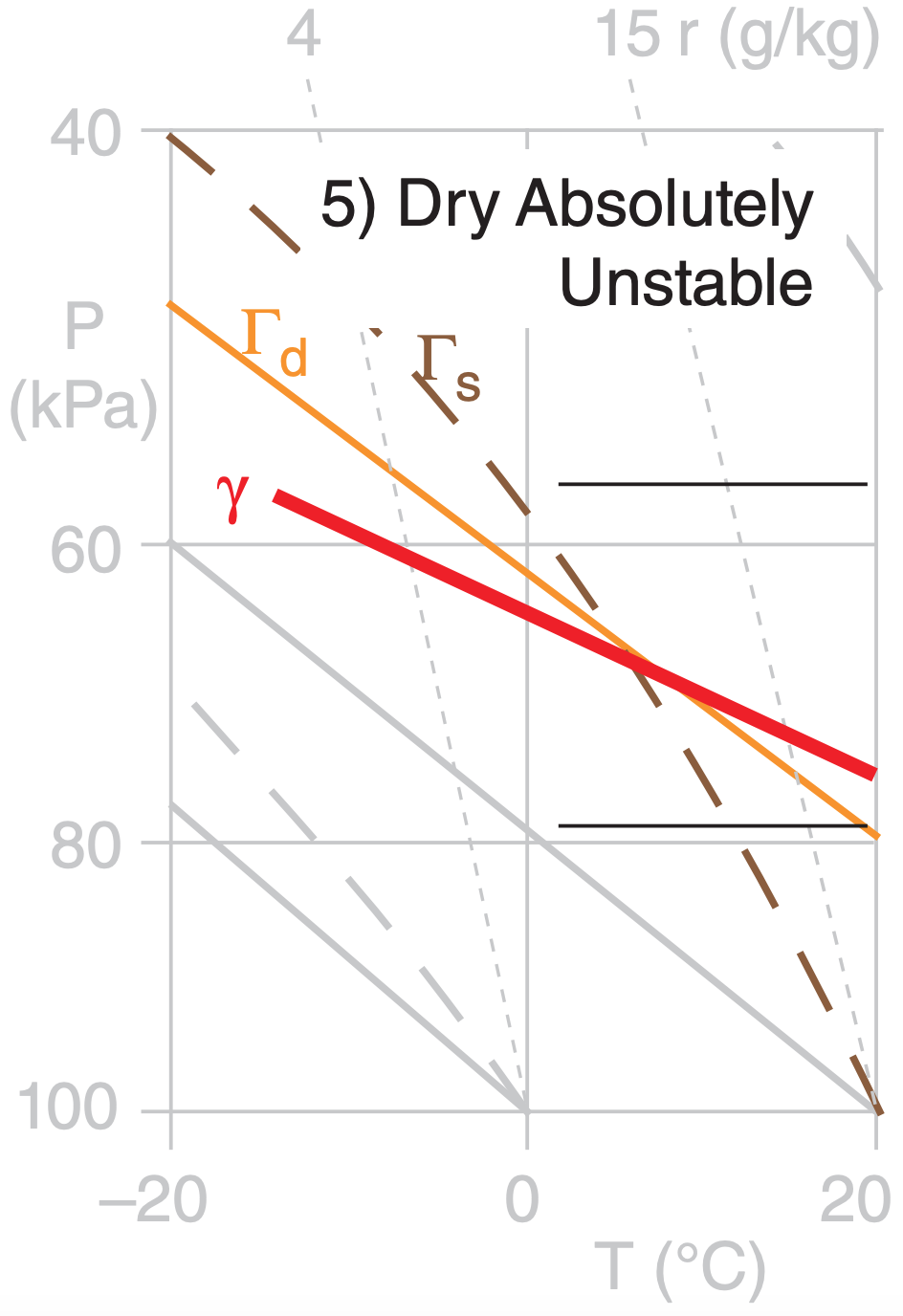
Layer Stability Classes: Five classes of layer stability are listed in Table 5-2. For a layer of air that is already saturated (namely, it is a layer of clouds, with T = Td ), then the environmental lapse rate γ, which is still defined by the equation above, is indicated as γs to remind us that the layer is saturated. As before, the word “dry” just means unsaturated here, so there could be moisture in the air.
| Table 5-2. Layer static stability, where Γd = 9.8°C km–1 is the dry adiabatic lapse rate, and Γs is the saturated adiabatic lapse rate. Γs is always ≤ Γd . | |
| Name | Layer Lapse Rate |
|---|---|
| 1) absolutely stable | γ < Γs |
| 2) saturated neutral | γs = Γs |
| 3) conditionally unstable | Γs < γ < Γd |
| 4) dry neutral | γ = Γd |
| 5) dry absolutely unstable | γ > Γd |
Figure 5.15 illustrates these stabilities. The layer of air between the thin horizontal lines has a linear lapse rate shown by the thick line. The slope of this thick line relative to the slopes of the dry Γd and moist Γs adiabats determines the layer stability class.
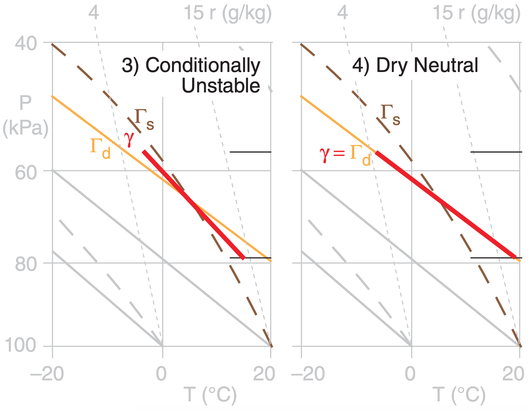
Conditional Stability: One of the types of layer stability listed in Table 5-2 is conditional stability. A layer of conditionally unstable air has lapse rate between the dry and moist adiabatic lapse rates. This layer is stable if the air is unsaturated, but is unstable if the air is saturated (cloudy). Hence, the “condition” refers to whether the air is cloudy or not.
Conditionally unstable air, if over a deep enough layer, is a favorable environment for thunderstorms to grow. A special set of thunderstorm stability indices has been developed to determine if thunderstorms will form, and how intense they might be. These are discussed in the Thunderstorm chapters of this book. The presence of thunderstorms indicate violently unstable air that extends throughout the depth of the troposphere.
When a whole layer is lifted, the temperature at each level within that layer will change according to whether those levels are saturated or not. Figure 5.16 shows a sample sounding, and how temperatures change following dry adiabats until reaching their local LCL, above which they follow the moist adiabat. This particular example shows how a layer that starts as conditionally unstable can become absolutely unstable if the bottom of the layer reaches saturation sooner than the top.
Nonetheless, I recommend that you use the parcel method to determine static stability. Even a stable layer can become turbulent (i.e., unstable) if buoyant air parcels move through it nonlocally.
5.7.2. Dynamic Stability
Dynamic stability considers both buoyancy and wind shear to determine whether the flow will become turbulent. Wind shear is the change of wind speed or direction with height, and can be squared to indicate the kinetic energy available to cause turbulence.
The ratio of buoyant energy to shear-kinetic energy is called the bulk Richardson number, Ri, which is dimensionless:
\(\ \begin{align} R i=\frac{|g| \cdot\left(\Delta T_{v}+\Gamma_{d} \cdot \Delta z\right) \cdot \Delta z}{T_{v} \cdot\left[(\Delta U)^{2}+(\Delta V)^{2}\right]}\tag{5.9a}\end{align}\)
and
\(\ \begin{align} R i=\frac{|g| \cdot \Delta \theta_{v} \cdot \Delta z}{T_{v} \cdot\left[(\Delta U)^{2}+(\Delta V)^{2}\right]}\tag{5.9b}\end{align}\)
where [ ∆θv, ∆U, ∆V, ∆Tv ] are the change of [virtual potential temperature, east-west wind component, north-south wind component, virtual temperature] across a layer of thickness ∆z. As before, Γd = 9.8 ·K km–1 is the dry adiabatic lapse rate, and Tv must be in absolute units (K) in the denominator of eq. (5.9).
Sample Application
Given these data, is the atmosphere turbulent?
| z (km) | Tv (°C) | U (m s–1) | V (m s–1) |
| 5.5 | –23 | 50 | 0 |
| 5.0 | –20 | 40 | 8 |
Find the Answer
Given: ∆T = –3°C, ∆V = –8, ∆U = 10 m s–1, ∆z = 0.5 km, where all vertical differences are (top – bottom)
Find: Turbulent (yes/no) ?
First, examine static stability.
∆θv = ∆Tv + Γd·∆z = ( –3°C) + (9.8 °C km–1)·(0.5 km) = 1.9°C
Because the top of the layer has warmer θv than the bottom, the air is locally statically stable. No nonlocal info to alter this conclusion. Thus, static stability does not make the air turbulent. But need to consider wind.
Apply eq. (5.9b). Use average Tv = –21.5+273 = 251.5 K
\(R i=\frac{\left(9.8 \mathrm{m} \cdot \mathrm{s}^{-2}\right) \cdot(1.9 \mathrm{K}) \cdot(500 \mathrm{m})}{(251.5 \mathrm{K}) \cdot\left[(10)^{2}+(-8)^{2}(\mathrm{m} / \mathrm{s})^{2}\right]}=0.226\)
This Ri below the critical value of 0.25, therefore the flow is turbulent because of dynamic instability.
Check: Physics are reasonable. Ri is dimensionless.
Exposition: Turbulence tends to mix the air, which reduces wind shears and temperature differences, and thus undoes the dynamic instability that caused it, as expected by LeChatelier’s Principle (see INFO box).
For the special case of statically stable air:
\(\ \begin{align} R i=\frac{N_{B V}^{2} \cdot(\Delta z)^{2}}{(\Delta U)^{2}+(\Delta V)^{2}}\tag{5.9c}\end{align}\)
NBV is undefined for air that is not statically stable.
For thin layers of atmosphere, the system is dynamically unstable if
\(\ \begin{align} R i<R i_{c}\tag{5.10}\end{align}\)
Ric = 0.25 is the critical Richardson number.
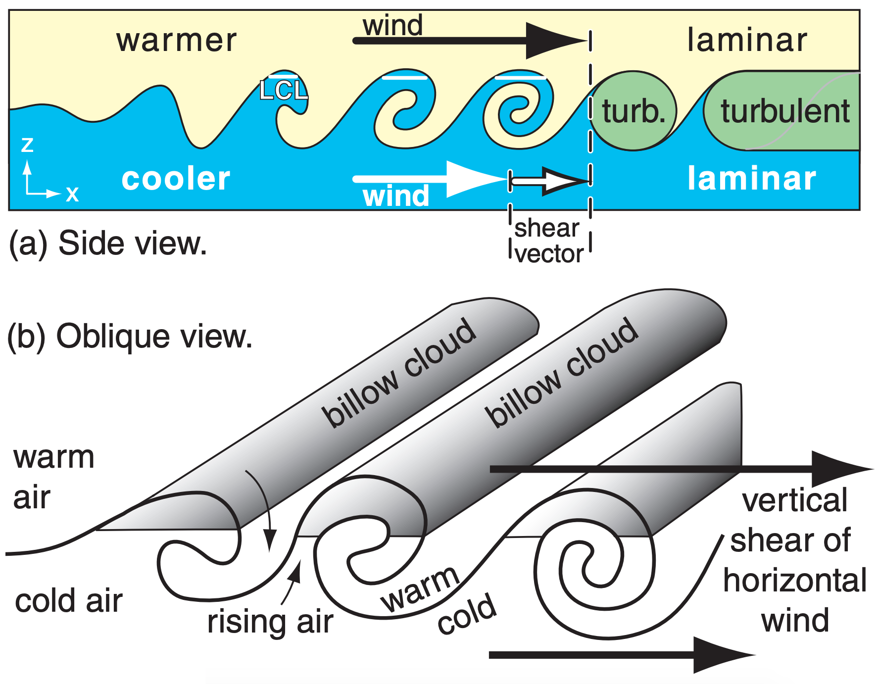
When statically stable laminar flow is just becoming dynamically unstable due to an increase in wind shear, the dynamically unstable layer behaves like breaking ocean waves (Figure 5.17) in slow motion. These waves are called Kelvin-Helmholtz waves, or K-H waves for short. As these waves break, the dynamically unstable layer becomes turbulent, and is known as clear-air turbulence (CAT) if outside thunderstorms and above the boundary layer.
If the bottom layer of cool air is humid enough, then clouds can form in any wave crest that is higher than its lifting condensation level (LCL). Since these clouds form narrow parallel bands perpendicular to the shear vector, the clouds look like billows of an accordion, and are called billow clouds (Figure 5.17).
5.7.3. Existence of Turbulence
Statically stable flows can be dynamically unstable and can become turbulent if the wind shear is strong enough.
Nonlocally statically unstable flow always becomes turbulent regardless of the wind shear. Thus, either dynamic instability or nonlocal static instability are sufficient to enable turbulence.
However, laminar flow exists only if the layer of air is stable both dynamically and statically.
Sample Application
For the following sounding, determine the regions of turbulence.
| z (km) | T (°C) | U (m s–1) | V (m s–1) |
| 2 | 0 | 15 | 0 |
| 1.5 | 0 | 12 | 0 |
| 1.2 | 2 | 6 | 4 |
| 0.8 | 2 | 5 | 4 |
| 0.1 | 8 | 5 | 2 |
| 0 | 12 | 0 | 0 |
Find the Answer
Given: The sounding above.
Find: a) Static stability (nonlocal parcel apex method), b) dynamic stability, & (c) identify turbulence.
Assume dry air, so T = Tv.
Method: Use spreadsheet to compute θ and Ri. Note that Ri applies to the layers between sounding levels.
| z (km) | θ (°C) | zlayer (km) | Ri |
| 2 | 19.6 | ||
| 1.5 | 14.7 | 1.5 to 2.0 | 9.77 |
| 1.2 | 13.8 | 1.2 to 1.5 | 0.19 |
| 0.8 | 9.8 | 0.8 to 1.2 | 55.9 |
| 0.1 | 9.0 | 0.1 to 0.8 | 5.25 |
| 0 | 12 | 0 to 0.1 | –0.358 |
Next, plot these results:
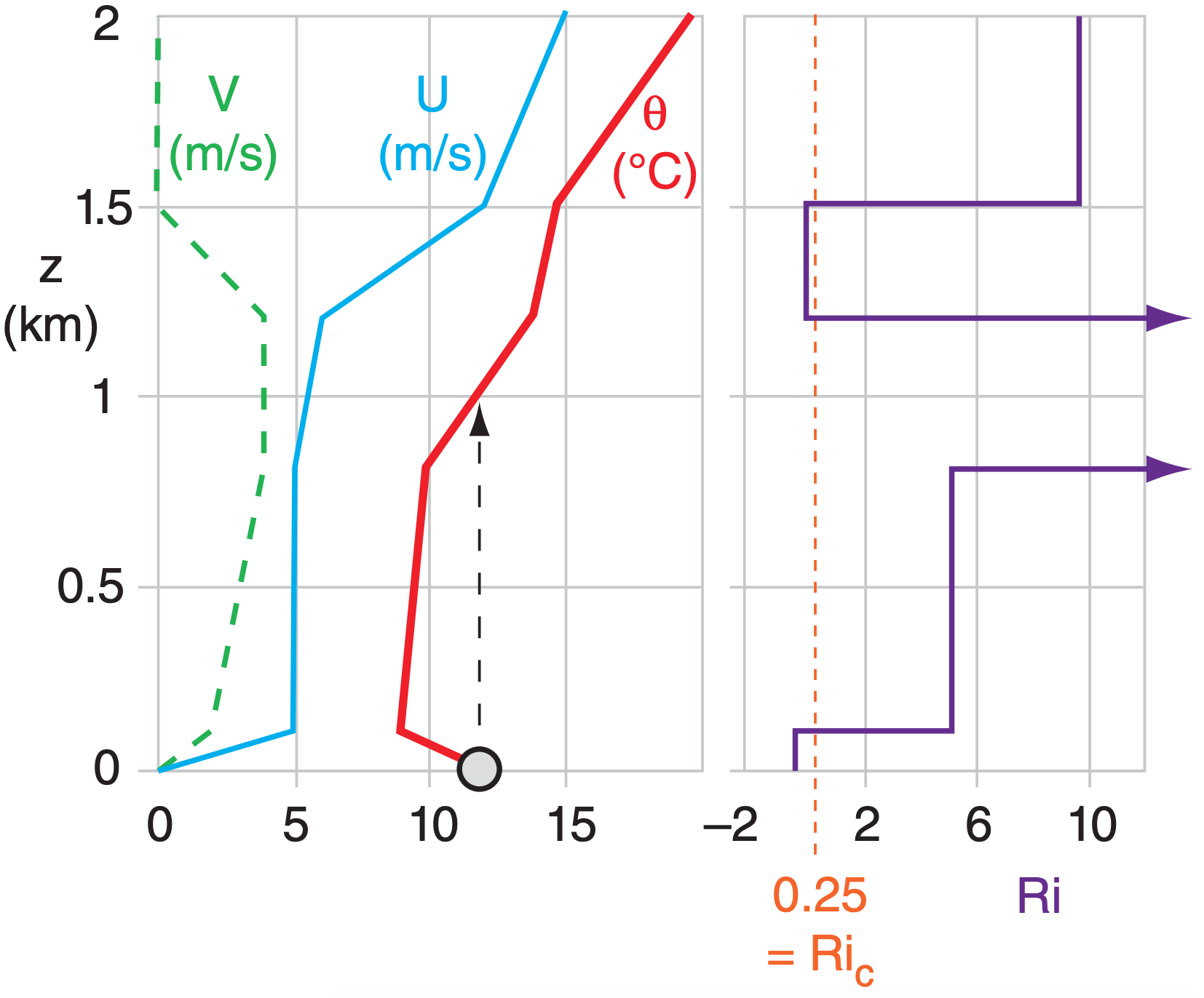
a) Static Stability: Unstable & turbulent for z = 0 to 1 km, as shown by nonlocal air-parcel rise in the θ sounding.
b) Dynamic Stability: Unstable & turbulent for z = 0 to 0.1 km, & for z = 1.2 to 1.5 km, where Ri < 0.25.
c) Turbulence exists where the air is statically OR dynamically unstable, or both. Therefore: Turbulence at 0 - 1 km, and 1.2 to 1.5 km.
Check: Physics, sketch & units are reasonable.
Exposition: At z = 0 to 1 km is the mixed layer (a type of atmos. boundary layer). At z = 1.2 to 1.5 is clear-air turbulence (CAT) and perhaps K-H waves.