4.1: Moisture Variables
- Page ID
- 9548
\( \newcommand{\vecs}[1]{\overset { \scriptstyle \rightharpoonup} {\mathbf{#1}} } \)
\( \newcommand{\vecd}[1]{\overset{-\!-\!\rightharpoonup}{\vphantom{a}\smash {#1}}} \)
\( \newcommand{\id}{\mathrm{id}}\) \( \newcommand{\Span}{\mathrm{span}}\)
( \newcommand{\kernel}{\mathrm{null}\,}\) \( \newcommand{\range}{\mathrm{range}\,}\)
\( \newcommand{\RealPart}{\mathrm{Re}}\) \( \newcommand{\ImaginaryPart}{\mathrm{Im}}\)
\( \newcommand{\Argument}{\mathrm{Arg}}\) \( \newcommand{\norm}[1]{\| #1 \|}\)
\( \newcommand{\inner}[2]{\langle #1, #2 \rangle}\)
\( \newcommand{\Span}{\mathrm{span}}\)
\( \newcommand{\id}{\mathrm{id}}\)
\( \newcommand{\Span}{\mathrm{span}}\)
\( \newcommand{\kernel}{\mathrm{null}\,}\)
\( \newcommand{\range}{\mathrm{range}\,}\)
\( \newcommand{\RealPart}{\mathrm{Re}}\)
\( \newcommand{\ImaginaryPart}{\mathrm{Im}}\)
\( \newcommand{\Argument}{\mathrm{Arg}}\)
\( \newcommand{\norm}[1]{\| #1 \|}\)
\( \newcommand{\inner}[2]{\langle #1, #2 \rangle}\)
\( \newcommand{\Span}{\mathrm{span}}\) \( \newcommand{\AA}{\unicode[.8,0]{x212B}}\)
\( \newcommand{\vectorA}[1]{\vec{#1}} % arrow\)
\( \newcommand{\vectorAt}[1]{\vec{\text{#1}}} % arrow\)
\( \newcommand{\vectorB}[1]{\overset { \scriptstyle \rightharpoonup} {\mathbf{#1}} } \)
\( \newcommand{\vectorC}[1]{\textbf{#1}} \)
\( \newcommand{\vectorD}[1]{\overrightarrow{#1}} \)
\( \newcommand{\vectorDt}[1]{\overrightarrow{\text{#1}}} \)
\( \newcommand{\vectE}[1]{\overset{-\!-\!\rightharpoonup}{\vphantom{a}\smash{\mathbf {#1}}}} \)
\( \newcommand{\vecs}[1]{\overset { \scriptstyle \rightharpoonup} {\mathbf{#1}} } \)
\( \newcommand{\vecd}[1]{\overset{-\!-\!\rightharpoonup}{\vphantom{a}\smash {#1}}} \)
\(\newcommand{\avec}{\mathbf a}\) \(\newcommand{\bvec}{\mathbf b}\) \(\newcommand{\cvec}{\mathbf c}\) \(\newcommand{\dvec}{\mathbf d}\) \(\newcommand{\dtil}{\widetilde{\mathbf d}}\) \(\newcommand{\evec}{\mathbf e}\) \(\newcommand{\fvec}{\mathbf f}\) \(\newcommand{\nvec}{\mathbf n}\) \(\newcommand{\pvec}{\mathbf p}\) \(\newcommand{\qvec}{\mathbf q}\) \(\newcommand{\svec}{\mathbf s}\) \(\newcommand{\tvec}{\mathbf t}\) \(\newcommand{\uvec}{\mathbf u}\) \(\newcommand{\vvec}{\mathbf v}\) \(\newcommand{\wvec}{\mathbf w}\) \(\newcommand{\xvec}{\mathbf x}\) \(\newcommand{\yvec}{\mathbf y}\) \(\newcommand{\zvec}{\mathbf z}\) \(\newcommand{\rvec}{\mathbf r}\) \(\newcommand{\mvec}{\mathbf m}\) \(\newcommand{\zerovec}{\mathbf 0}\) \(\newcommand{\onevec}{\mathbf 1}\) \(\newcommand{\real}{\mathbb R}\) \(\newcommand{\twovec}[2]{\left[\begin{array}{r}#1 \\ #2 \end{array}\right]}\) \(\newcommand{\ctwovec}[2]{\left[\begin{array}{c}#1 \\ #2 \end{array}\right]}\) \(\newcommand{\threevec}[3]{\left[\begin{array}{r}#1 \\ #2 \\ #3 \end{array}\right]}\) \(\newcommand{\cthreevec}[3]{\left[\begin{array}{c}#1 \\ #2 \\ #3 \end{array}\right]}\) \(\newcommand{\fourvec}[4]{\left[\begin{array}{r}#1 \\ #2 \\ #3 \\ #4 \end{array}\right]}\) \(\newcommand{\cfourvec}[4]{\left[\begin{array}{c}#1 \\ #2 \\ #3 \\ #4 \end{array}\right]}\) \(\newcommand{\fivevec}[5]{\left[\begin{array}{r}#1 \\ #2 \\ #3 \\ #4 \\ #5 \\ \end{array}\right]}\) \(\newcommand{\cfivevec}[5]{\left[\begin{array}{c}#1 \\ #2 \\ #3 \\ #4 \\ #5 \\ \end{array}\right]}\) \(\newcommand{\mattwo}[4]{\left[\begin{array}{rr}#1 \amp #2 \\ #3 \amp #4 \\ \end{array}\right]}\) \(\newcommand{\laspan}[1]{\text{Span}\{#1\}}\) \(\newcommand{\bcal}{\cal B}\) \(\newcommand{\ccal}{\cal C}\) \(\newcommand{\scal}{\cal S}\) \(\newcommand{\wcal}{\cal W}\) \(\newcommand{\ecal}{\cal E}\) \(\newcommand{\coords}[2]{\left\{#1\right\}_{#2}}\) \(\newcommand{\gray}[1]{\color{gray}{#1}}\) \(\newcommand{\lgray}[1]{\color{lightgray}{#1}}\) \(\newcommand{\rank}{\operatorname{rank}}\) \(\newcommand{\row}{\text{Row}}\) \(\newcommand{\col}{\text{Col}}\) \(\renewcommand{\row}{\text{Row}}\) \(\newcommand{\nul}{\text{Nul}}\) \(\newcommand{\var}{\text{Var}}\) \(\newcommand{\corr}{\text{corr}}\) \(\newcommand{\len}[1]{\left|#1\right|}\) \(\newcommand{\bbar}{\overline{\bvec}}\) \(\newcommand{\bhat}{\widehat{\bvec}}\) \(\newcommand{\bperp}{\bvec^\perp}\) \(\newcommand{\xhat}{\widehat{\xvec}}\) \(\newcommand{\vhat}{\widehat{\vvec}}\) \(\newcommand{\uhat}{\widehat{\uvec}}\) \(\newcommand{\what}{\widehat{\wvec}}\) \(\newcommand{\Sighat}{\widehat{\Sigma}}\) \(\newcommand{\lt}{<}\) \(\newcommand{\gt}{>}\) \(\newcommand{\amp}{&}\) \(\definecolor{fillinmathshade}{gray}{0.9}\)Sample Application
For T = 10°C and P = 70 kPa, calculate qs, rs, & ρvs.
Find the Answer
Given: T = 10°C = 283.15 K, P = 70 kPa
Find: qs = ? g kg–1, rs = ? g kg–1, ρvs = ? g m–3
Get es = 1.232 kPa from Table 4-1 (independent of P).
Apply eq. (4.8) to get qs:
qs = 0.622·(1.232 kPa)/(70 kPa) = 0.0109 g g–1 ≈ 11 g kg–1
Apply eq. (4.12) to get ρvs:
ρvs = (1232. Pa)/[(461 J·K–1·kg–1)·(283.15 K)] = 0.00944 kg·m–3 = 9.44 g·m–3 .
Check: Physics and units are reasonable.
Exposition: Table 4-1 could have been used for ρvs .
Table 4-2 (continued across several pages) shows most of the moisture variables used in meteorology. Other variables used in the table below include: m = mass, e = vapor pressure, P = total atmospheric pressure, ℜd = 2.871x10⁻⁴ kPa·K–1·m3·g–1 is the gas constant for dry air, ℜv = 4.61x10⁻⁴ kPa·K–1·m3·g–1 is the gas constant for pure water vapor, Pd is the partial pressure of dry air, ρd is the density of dry air (which is a function of pressure, altitude and temperature as given by the ideal gas law), and subscript s denotes saturation.
| Table 4-2a. Moisture variables. | |||
| Variable name: | Mixing Ratio | Specific Humidity | Absolute Humidity |
|---|---|---|---|
| Symbol: | r | q | ρv |
| Units: | kgwater vapor kgdry air–1 | kgwater vapor kgtotal air–1 | kgwater vapor m–3 |
| Alternative Units: | g kg–1 , g g–1 , kg kg–1 | g kg–1 , g g–1 , kg kg–1 | kg m–3 |
| Defining Equation: (& equation number) | \(\ r=\frac{m_{\text{water vapor}}}{m_{\text{dry air}}} \) (4.3) |
\(\ q=\frac{m_{\text{water vapopr}}}{m_{\text{total air}}}\) (4.6) \(\ q=\frac{m_{\text{water vapor}}}{m_{\text{dry air }}+ m_{\text{water vapor}}}\) |
\(\ \rho_v=\frac{m_{\text{water vapor}}}{volume} \) (4.9) |
| Relationship to Vapor Pressure: | \(r=\frac{\varepsilon \cdot e}{P-e}\) (4.4) |
\(q=\frac{\varepsilon \cdot e}{P_{d}+\varepsilon \cdot e}=\frac{\varepsilon \cdot e}{P-e \cdot(1-\varepsilon)}\) (4.7) \(q \approx \frac{\varepsilon \cdot e}{P}\) |
\(\rho_{v}=\frac{e}{\mathfrak{R}_{v} \cdot T}\) (4.10) \(\rho_{v}=\frac{e \cdot \varepsilon \cdot \rho_{d}}{P-e} \approx \frac{e}{P} \cdot \varepsilon \cdot \rho_{d}\) (4.11) |
| If Saturated: | \(r_{S}=\frac{\boldsymbol{\varepsilon} \cdot e_{S}}{P-e_{S}}\) (4.5) |
\(q_{s}=\frac{\varepsilon \cdot e_{s}}{P_{d}+\varepsilon \cdot e_{s}}\) (4.8) \(q_{s}=\frac{\varepsilon \cdot e_{S}}{P-e_{S} \cdot(1-\varepsilon)} \approx \frac{\varepsilon \cdot e_{S}}{P}\) |
\(\rho_{v s}=\frac{e_{s}}{\mathfrak{R}_{v} \cdot T}\) (4.12) \(\rho_{v s}=\frac{e_{s} \cdot \varepsilon \cdot \rho_{d}}{P-e_{s}} \approx \frac{e_{s}}{P} \cdot \varepsilon \cdot \rho_{d}\) (4.13) |
| Key Constants: | \(\begin{aligned} \varepsilon &=\Re_{d} / \Re_{v} \\ &=0.622 \mathrm{g}_{\text {vapor }} \mathrm{g}_{\mathrm{dry \ air}} ^{-1} \\ &=622 \mathrm{g} \mathrm{kg}^{-1} \end{aligned}\) | \(\begin{aligned} \varepsilon &=\Re_{d} / \Re_{v} \\ &=0.622 \mathrm{g}_{\mathrm{vapor}} \mathrm{g}_{\mathrm{dry\ air}} ^{-1} \\ &=622 \mathrm{g} \mathrm{kg}^{-1} \end{aligned}\) | \(\begin{aligned} \Re_{v} &=4.61 \times 10^{-4} \\ & \mathrm{kPa} \cdot \mathrm{K}^{-1} \cdot \mathrm{m}^{3} \cdot \mathrm{g}^{-1} \\ \varepsilon &=622 \mathrm{g} \mathrm{kg}^{-1} \end{aligned}\) |
| Typical Values: | See Table 4-1. | See Table 4-1. | See Table 4-1. |
| Relevance: |
• r is conserved in unsaturated air parcels that move without mixing with their environment. • not affected by heating, cooling, pressure changes. • used in thermo diagrams. |
• q is conserved in unsaturated air parcels that move without mixing with their environment. • not affected by heating, cooling, pressure changes. |
• easy to measure using absorption of infrared, ultraviolet, or microwave radiation as a function of path length through the air. • is the concentration of water vapor in air |
| Notes: | Derivation of eq. (4.4): Given eq. (4.3), divide numerator and denominator by volume. But m/Volume is density. Use ideal gas laws for water vapor and for dry air, assuming a common T. | Derivation of eq. (4.7) is similar to that for eq. (4.4). |
• Eq. (4.10) is the ideal gas law for water vapor. • Eq. (4.11) uses the ideal gas law for dry air to replace temperature T. • T must be in Kelvin. |
| Table 4-2b. Moisture variables. | ||
| Variable name: | Relative Humidity | Dewpoint |
|---|---|---|
| Symbol: | RH or RH% | Td |
| Units: | (dimensionless) | (K) |
| Alternative Units: | (%) | (°C) |
| Defining Equation: (& equation number) | \(R H=\frac{e}{e_{S}} \quad\) or \(\quad \frac{R H \%}{100 \%}=\frac{e}{e_{S}}\) (4.14a) | “Temperature to which a given air parcel must be cooled at constant pressure and constant water-vapor content in order for saturation to occur.”* |
| Alternative Definitions: |
\(R H=\frac{q}{q_{s}}=\frac{\rho_{v}}{\rho_{v s}} \approx \frac{r}{r_{s}}\) (4.14b) \(\frac{R H \%}{100 \%}=\frac{q}{q_{s}}=\frac{\rho_{v}}{\rho_{v s}} \approx \frac{r}{r_{s}}\) (4.14c) |
\(T_{d}=\left[\frac{1}{T_{o}}-\frac{\Re_{v}}{L} \cdot \ln \left(\frac{e}{e_{o}}\right)\right]^{-1}\) (4.15a) \(T_{d}=\left[\frac{1}{T_{o}}-\frac{\Re_{v}}{L} \ln \left(\frac{r \cdot P}{e_{o} \cdot(r+\varepsilon)}\right)\right]^{-1}\) (4.15b) |
| If Saturated: | RH = 1.0 or RH% = 100% (4.14d) | Td = T |
| Key Constants: | eo = 0.6113 kPa, To = 273.15 K ℜv/Lv =1.844x10⁻⁴ K–1. | |
| Typical Values: | RH = 0.0 to 1.0 or RH% = 0% to 100% | See Table 4-1. Td ≤ T |
| Relevance: |
• regulates the max possible evaporation into the air. • easy to measure via: (1) capacitance changes across a plastic dielectric; (2) electrical resistance of an emulsion made of carbon powder; or (3) organic-fiber contraction/expansion. • most used by the general public. |
• easy to measure via cooling a mirror to the point where condensation (dew) forms on it. The temperature at which this first happens is the dewpoint, as detected by measuring how well a light beam can reflect off the mirror. • a very accurate method for humidity measurement. |
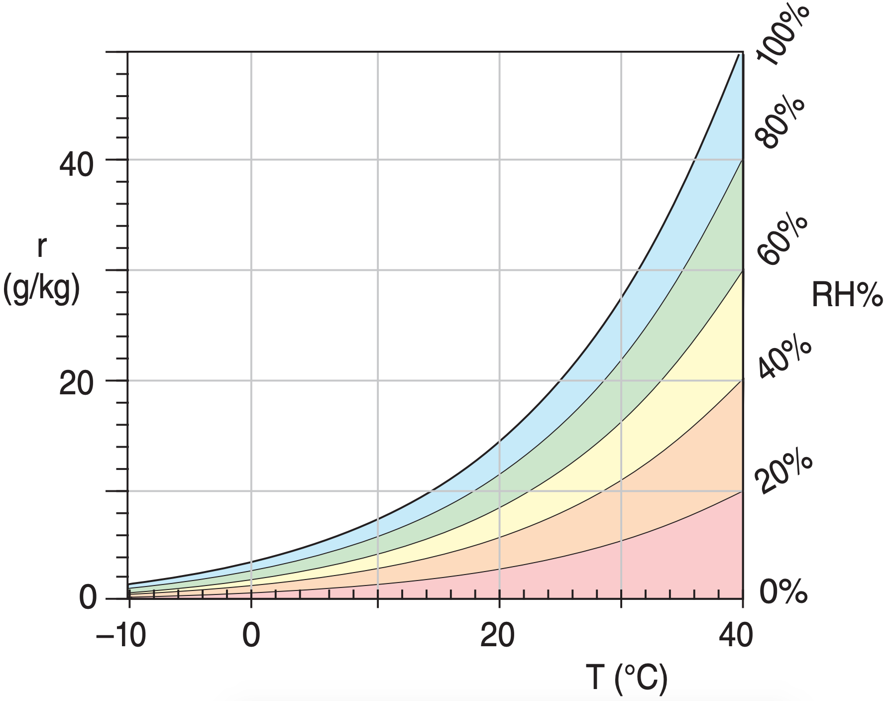
| Notes: | • it is possible to have relative humidities as high as about 100.5%. This is called supersaturation (see the Precipitation Processes chapter). See Figure 4.3 for RH% vs. r. |
• Td also called dewpoint temperature. • (T - Td) = dewpoint depression = temperature dewpoint spread * Glickman, T. S., 2000: Glossary of Meteorology. American Meteorological Society. |

Sample Application
Find Td and RH% for r= 10 g kg–1, P= 80 kPa, T=20°C.
Find the Answer
Given: r = 0.01 gvapor gair–1, P = 80 kPa, T = 20°C
Find: Td = ? °C, and RH% = ? %
Use eq. (4.15b): Td = [(1/(273.15K) – (1.844x10⁻⁴ K–1)·
ln{ [(80kPa)·(0.01gvapor gair–1)] / [(0.6113kPa)·((0.01g g–1) +(0.622g g–1)] }]–1 =[(1/(273.15K) – (1.844x10⁻⁴K–1)·ln(2.07)]–1 = 283.78K
Thus, Td = 283.78 – 273.15 = or 10.6°C
At Td = 10.6°C, eq. 4.1b gives e ≈ 1.286 kPa
At T = 20°C, Table 4-1 gives es = 2.369 kPa
Use eq. (4.14a): RH% = 100%·(1.286 kPa/2.369 kPa)
RH% = 54.3%
Check: Magnitude and units are reasonable.
| Table 4-2c. Moisture variables. | ||
| Variable name: | Lifting Condensation Level (LCL) | Wet-bulb Temperature |
|---|---|---|
| Symbol: | zLCL | Tw |
| Units: | (km) | (K) |
| Alternative Units: | (m) | (°C) |
| Defining Equation: (& equation number) | \(z_{L C L}=a \cdot\left(T-T_{d}\right)\) (4.16a) | \(C_{p} \cdot\left(T-T_{w}\right)=-L_{v} \cdot\left(r-r_{w}\right)\) (4.17) |
| Applications: | \(P_{L C L}=P \cdot\left[1-b \cdot\left(\frac{T-T_{d}}{T}\right)\right]^{C_{p} / \Re}\) (4.16b) |
\(r=r_{w}-\beta \cdot\left(T-T_{w}\right)\) (4.18a) where \(r_{w}=\frac{\varepsilon}{b \cdot P \cdot \exp \left(\frac{-c \cdot T_{w}\left(^{\circ} C\right)}{T_{w}\left(^{\circ} C\right)+\alpha}\right)-1}\) (4.18b) |
| If Saturated: | \(z_{L C L}=0 \quad, \quad P_{L C L}=P\) | \(T_{w}=T,\) for \(T=\) dry-bulb temperature |
| Key Constants: |
a = 0.125 km °C–1. Γd = 9.8 °C km–1 b = a·Γd = 1.225 (dimensionless) CP/ℜ = 3.5 (dimensionless) |
ε = 622 g kg–1, b = 1.631 kPa–1, c = 17.67, α = 243.5°C, β = 0.40224 (g kg–1)/°C. |
| Relevance: |
• for unsaturated air, it is the height (or pressure) to which air must be lifted to become just saturated (i.e., cloudy). • is cloud-base altitude for cumulus and other convective clouds. |
• easy to measure, by placing a wet wick or sleeve around a thermometer bulb, and then blowing air past the wet bulb (an aspirated psychrometer) or moving the wet bulb through the air (a sling psychrometer). |
| Notes: |
• does NOT give cloud base for stratiform clouds, because these clouds are caused by advection (nearly horizontal winds). • the LCL is also known as the saturation level. For saturated air, it is the height to which air must be lowered to become just unsaturated (eqs 4.16 do NOT apply). |
• as water evaporates from the wet wick, the adjacent air temperature drops from T to Tw while the humidity in this air increases from r to rw, until equilibrium heat balance is reached as described by eq. (4.17). • (T – Tw) is called wet-bulb depression. • see Normand’s rule on later pages. |
Sample Application
For an air parcel at P = 90 kPa with T = 25°C and Td = 8°C, what is the height and pressure of the LCL?
Find the Answer
Given: P = 90 kPa, T = 25°C = 298.15 K, Td = 8°C .
Find: zLCL = ? km , PLCL = ? kPa
Use eq. (4.16a)
zLCL = (0.125 km °C–1)·(25 – 8°C) = 2.13 km higher than the initial height.
Use eq. (4.16b)
PLCL = (90 kPa)·[1 – 1.225·(25–8°C)/298.15K]3.5 = 69.85 kPa
Check: Physics and units are reasonable.
Exposition: The pressure decreases about 10 kPa for each increase of 1 km of altitude near the surface, the pressure answer is also reasonable. Indeed, an air parcel moving from 90 to 70 kPa rises about 2 km.
Sample Application
You observe a dry-bulb (i.e., normal air) temperature of T = 25°C, and a wet-bulb temperature of 18°C. Use the equations to calculate the mixing ratio for P = 90 kPa. Don’t use look-up tables or graphs.
Find the Answer
Given: P = 90 kPa, T = 25°C , Tw = 18°C
Find: r = ? g kg–1
First, solve eq. (4.18b):
\(r_{w}=\frac{622 \mathrm{g} / \mathrm{kg}}{\left(1.631 \mathrm{kPa}^{-1}\right) \cdot(90 \mathrm{kPa}) \cdot \exp \left(\frac{-17.67 \cdot 18^{\circ} \mathrm{C}}{18^{\circ} \mathrm{C}+243.5^{\circ} \mathrm{C}}\right)-1}\)
rw = 14.6 g kg–1.
Then solve eq. (4.18a):
r = (14.6g kg–1) – [0.40224 (g kg–1)/°C]·(25–18°C) = 11.78 g kg–1.
Check: Physics and units are reasonable.
Exposition: Knowing r, use other eqs. to find any other humidity variable.
Sample Application
Find the mixing ratio and relative humidity for air temperature of 12°C and wet-bulb temperature of 10°C. Yes, you may use the graphs this time.
Find the Answer
Given: T = 12°C , Tw = 10°C
Find: r = ? g kg–1 , and RH = ? %
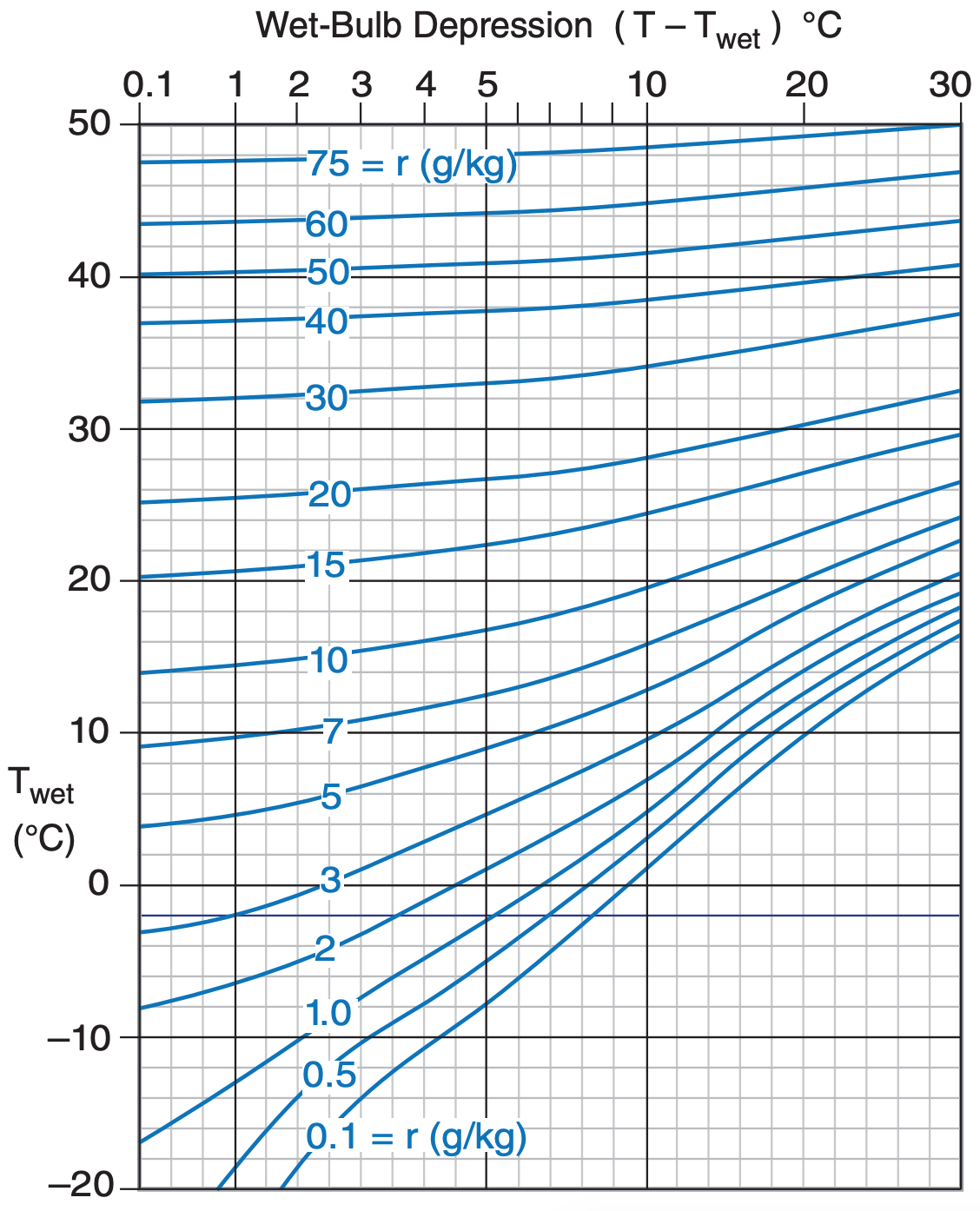
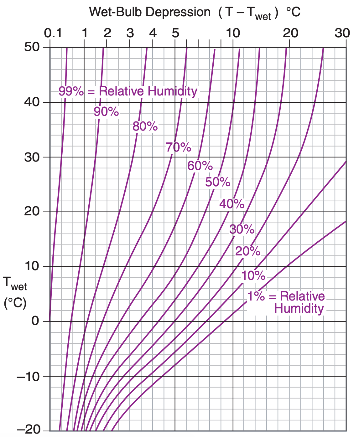
Assume P = 101.3 kPa, so we can use Figs. 4.4 & 4.5.
The wet-bulb depression is 12 – 10 = 2°C
Use Figure 4.4. r = 7 g kg–1.
Use Figure 4.5. RH = 78% .
Check: Physics and units are reasonable.
Exposition: Much easier than the Sample Applications on the previous page. Notice that in Figure 4.4, r depends mostly on Tw, because the mixing-ratio lines are mostly horizontal. However, RH% depends mostly on T – Tw , because the lines in Figure 4.5 are mostly vertical.
4.2.1. More Wet-bulb Temperature Info
The easiest way for you to find humidity from dry and wet-bulb temperature is to look-up the humidity in tables called psychrometric tables, which are often published in meteorology books. Figures 4.4 and 4.5 present the look-up information as psychrometric graphs, which were computed from the equations in this Chapter.
To create your own psychrometric tables or graphs, first generate a table of mixing ratios in a spreadsheet program, using eqs. (4.18a) and (4.18b). I assumed a standard sea-level pressure of P = 101.325 kPa for the figures here. Then contour the resulting numbers to give Figure 4.4. Starting with the table of mixing ratios, use eqs. (4.2), (4.5), and (4.14b or c) to create a new table of relative humidities, and contour it to give Figure 4.5. All of these psychrometric tables and graphs are based on Tetens’ formula (see eq. 4.2).


It is easy to calculate other humidity variables such as mixing ratio or relative humidity from known values of T and Tw. Eqs. (4.18) and Figs 4.4 and 4.5 are examples of this.
However, going the opposite way is more difficult. If you are given other humidity variables it is hard to find the wet-bulb temperature. Namely, to use the equations or figures mentioned above, you would need to iterate to try to converge on the correct answer.
Instead, there are two methods to estimate Tw. One is an empirical approximation (given below), and the other is a graphical method called Normand’s Rule (given on the next page).
The empirical approximation for Tw (in °C) at sea level is a function of air temperature T (in °C) and relative humidity RH% (e.g., using 65.8 to represent 65.8%):
\(\begin{align} T_{w} \approx T \cdot \operatorname{atan}\left[0.151977(R H \%+8.313659)^{1 / 2}\right]-4.686035 +\operatorname{atan}(T+R H \%)-\operatorname{atan}(R H \%-1.67631)+0.00391838 \cdot(R H \%)^{3 / 2} \cdot \operatorname{atan}\left(0.023101 \cdot R H^{\%}\right) \tag{4.19}\end{align}\)
where the arctangent (atan) function returns values in radians. [CAUTION: If your software returns arctangent values in degrees, be sure to convert to radians before you use them in the equation above.]
Sample Application
Given an air temperature of 20°C and a relative humidity of 50%, use the empirical method to estimate the wet-bulb temperature at sea level.
Find the Answer
Given: T = 20°C , RH% = 50
Find: Tw = ? °C
Apply eq. (4.19):
Tw = 20 . arctan[0.151977 . (50 + 8.313659)1/2] + arctan(20+50) - arctan(50-1.676331) + 0.00391838 . (50)3/2 . arctan(0.023101.50) - 4.686035
Tw = 13.7 °C
Check: Units reasonable. Agrees with Figure 4.5.
Exposition: Although this equation had many terms, it needed to be solved only once. Contrast this with iterative methods, which require repeated solutions of equations in order to converge to an answer
Sample Application
The air temperature is T = 20°C and the mixing ratio is 7.72 g/kg (which you might have found using a psychrometer with a wet-bulb temperature of 14°C). Use the equations to calculate the relative humidity for P = 100 kPa. Don’t use look-up tables or graphs.
Find the Answer
Given: T = 20°C , r = 7.72 g kg–1, P = 100 kPa
Find: RH = ? %
First, use Tetens’ formula (4.2), with the trick that ΔT = T(K) – T1(K) = [T(°C)+273.15] – 273.15 = T(°C) , and remembering that for temperature differences: 1°C = 1 K .
\(e_{s}=0.611(\mathrm{kPa}) \cdot \exp \left[\frac{17.2694 \cdot(20 \mathrm{K})}{(20+273.15) \mathrm{K}-35.86 \mathrm{K}}\right]\)
es = 2.34 kPa.
Next, use this in eq. (4.5):
\(r_{s}=\frac{(622 \mathrm{g} / \mathrm{kg}) \cdot 2.34 \mathrm{kPa}}{[100.0-2.34] \mathrm{kPa}}=14.9 \mathrm{g} / \mathrm{kg}\)
Finally, use eq. (4.14): RH = 100%·(r/rs)
RH = 100% · (7.72/14.9) = 51.8%
Check: Physics and units are reasonable.
Exposition: What a lot of work. If we instead had used psychrometric graph (Figure 4.5) with Tw = 14°C and T – Tw = 6°C , we would have found almost the same relative humidity much more easily.
Sample Application
For air of T = 25°C and Td = 18°C at P = 100 kPa, find Tw. Use Γs = 4.42 °C km–1 in Normand’s Rule.
Find the Answer
Given: P = 100 kPa, T = 25°C, Td = 18°C, Γs = 4.42 °C km–1
Find: Tw = ?°C
According to Normand’s Rule:
First, use eq. (4.16):
zLCL = (0.125 km °C–1)·(25 – 18°C) = 0.875 km.
Next, use eq. (4.20):
TLCL = 25 – (9.8 K km–1)·(0.875 km) = 16.43 °C.
Finally, use eq. (4.21):
Tw = 16.43 + (4.42 °C km–1)·(0.875 km) = 20.3°C.
Check: Physics and units are reasonable.
Exposition: The resulting wet-bulb depression is (T – Tw) = 4.7°C.
You can obtain Tw from Td via Normand’s Rule:
- First: Find zLCL using eq. (4.16).
- Next: \(\ \begin{align} T_{L C L}=T-\Gamma_{d} \cdot z_{L C L}\tag{4.20}\end{align}\)
- Finally: \(\ \begin{align}T_{w}=T_{L C L}+\Gamma_{s} \cdot z_{L C L}\tag{4.21}\end{align}\)
where the dry lapse rate is Γd = 9.8 K km–1 and the moist (saturated) lapse rate is Γs (magnitude varies, as explained later in this chapter). If you hypothetically lift an air parcel to its lifting condensation level, then its new temperature is TLCL. The wet-bulb temperature is always constrained between the drybulb temperature and the dew point: Td ≤ Tw ≤ T.
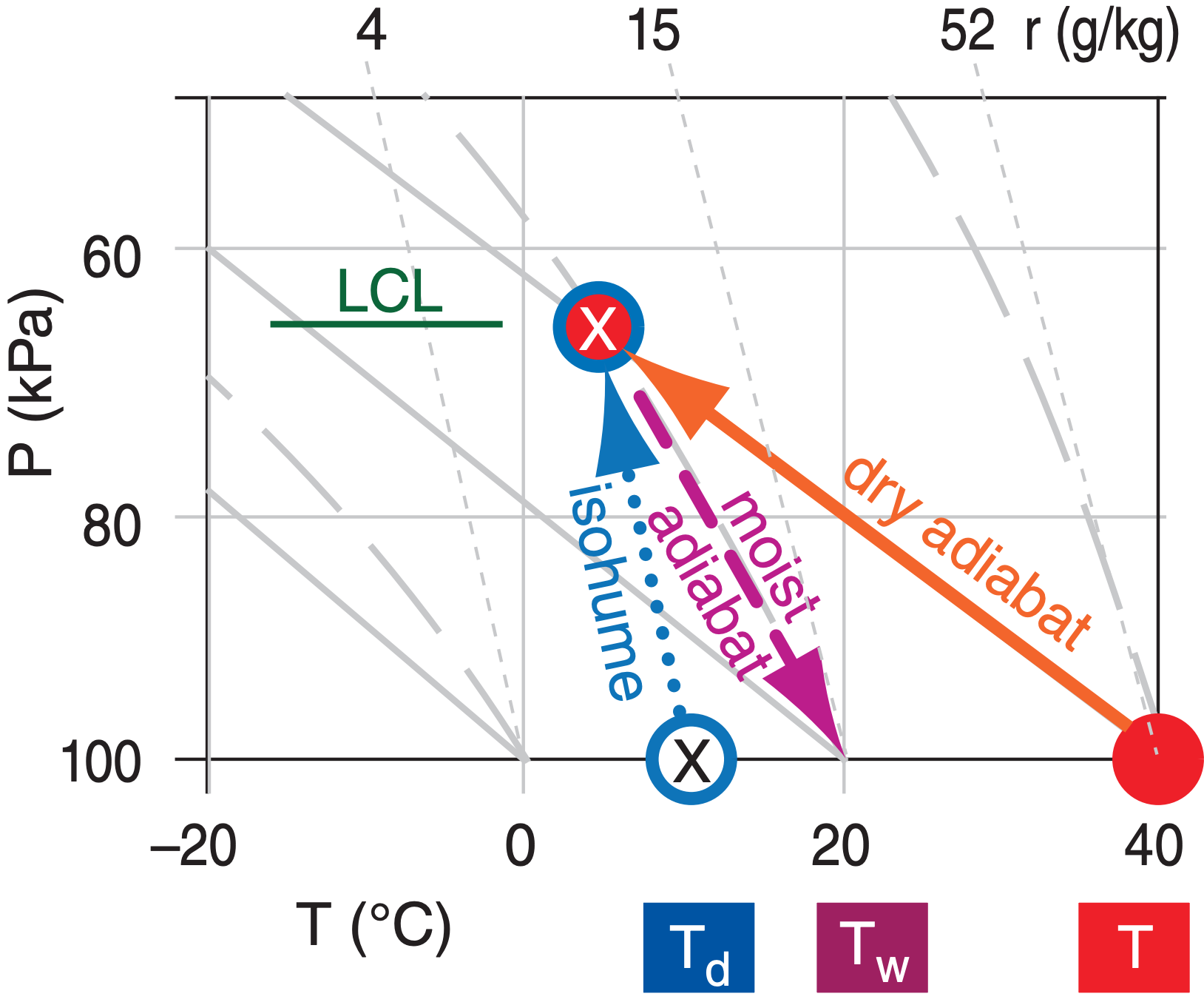
Normand’s rule is easy to implement on a thermo diagram. Although isohumes and moist adiabats on thermo diagrams are not introduced until later in this chapter, I demonstrate Normand’s rule here for future reference. Follow a dry adiabat up from the given dry-bulb temperature T, and follow an isohume up from the given dew point Td (Figure 4.6). At the LCL (where these two isopleths cross), follow a moist adiabat back down to the starting pressure to give the wet-bulb temperature Tw.

e = vapor pressure (kPa)
r = mixing ratio (g kg–1)
q = specific humidity (g kg–1)
ρv = absolute humidity (g m–3)
RH = relative humidity (%)
zLCL = lifting condensation level (km)
Td = dewpoint (temperature) (°C)
Tw = wet-bulb temperature (°C)
Notes:
- subscript s denotes saturation.
- most thermodynamic equations require temperatures to be converted into Kelvin.
- most thermo eqs. require mixing ratio in g g–1.
4.2.2. Converting Between Humidity Variables
Be sure to use g g–1 for q and r in the following equations:
\(\ \begin{align}q=\frac{r}{1+r}\tag{4.22}\end{align}\)
\(\ \begin{align}q=\frac{\rho_{v}}{\rho_{d}+\rho_{v}}\tag{4.23}\end{align}\)
\(\ \begin{align}q=\left(\frac{\varepsilon \cdot e_{0}}{P}\right) \cdot \exp \left[\frac{L}{\Re_{v}} \cdot\left(\frac{1}{T_{o}}-\frac{1}{T_{d}}\right)\right]\tag{4.24}\end{align}\)
\(\ \begin{align}e=\frac{r}{\varepsilon+r} \cdot P\tag{4.25}\end{align}\)
\(\ \begin{align}r=\frac{\rho_{v}}{\rho_{d}}\tag{4.26}\end{align}\)
Also, when humidities are not high:
\(\ \begin{align}r \approx q\tag{4.27a}\end{align}\)
\(\ \begin{align}r_{s} \approx q_{s}\tag{4.27b}\end{align}\)


