3.4: Heat Budget of an Unsaturated Air Parcel
- Page ID
- 9543
In this chapter, we consider a special case: unsaturated air parcels, for which no liquid or solid water is involved. The word “dry” is used to imply that phase changes of water are not considered. Nonetheless, the air CAN contain water vapor. In the next chapter we include the effects of saturation and possible phase changes in a “moist” analysis.
3.4.1. Lagrangian Form of the First Law of Thermo
The pressure of an air parcel usually equals that of its surrounding environment, which decreases exponentially with height. Thus, the last term of eq. (3.2d) will be non-zero for a rising or sinking air parcel as its pressure changes to match the pressure of its environment. But the pressure change with height was given by the hydrostatic equation in Chapter 1: ∆P/ρ = – |g| · ∆z. We can use this to rewrite the First Law of Thermo in the Lagrangian framework of a moving air parcel:
\(\ \begin{align}\Delta T=-\left(\frac{|g|}{C_{p}}\right) \cdot \Delta z+\frac{\Delta q}{C_{p}}\tag{3.5}\end{align}\)
Sample Application
A 5 kg air parcel of initial temperature 5°C rises 1 km and thermally loses 15 kJ of energy due to IR radiation. What is the final temperature of the parcel?
Find the Answer
Given: ∆Q = –15,000 J, mair = 5 kg, ∆z = 1000 m ,
Find: T = ? K
Convert from energy to energy/mass:
∆q = ∆Q/mair = (–15000 J)/(5 kg) = –3000 J kg–1 .
With lack of humidity info, assume dry air.
Cp = 1004. J·kg–1·K–1 (= units m2 s–2 K–1)
Apply eq. (3.5):
∆T = –[(9.8 m s–2)/ (1004 m2 s–2 K–1)]·(1000m) + [(–3000 J kg–1) / (1004. J·kg–1·K–1)] = (– 9.76 – 3.00) K = –12.76 °C
Check: Physics & units are reasonable.
Exposition: Because we are working with a temperature difference, recall that 1 K of temperature difference = 1°C of temperature difference. Hence, we could replace the Kelvin units with °C. The net result is that the rising air parcel cools due to both IR radiative cooling and work done on the atmosphere as the parcel rises.
Various processes can cause heat transfer (∆q). The sun could heat the air, or IR radiation could cool the air. Water vapor could condense and release its latent heat back into sensible heat. Exothermic chemical reactions or radioactive decay could occur among air pollutants carried within the parcel. Internal turbulence could dissipate into heat. Molecular conduction in the air is very weak, but turbulence could mix warmer or cooler air into the air parcel. Other processes such as convection and advection (Figure 3.2) do not change the parcel’s temperature, but can move the air parcel along with the heat that it possesses.
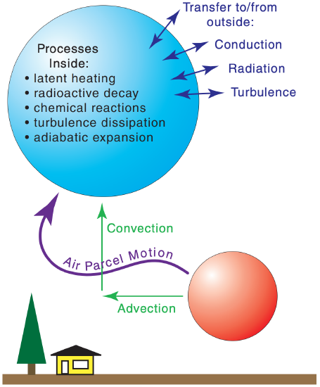
Eq. (3.5) represents a heat budget. Namely, parcel temperature (which indicates heat possessed) is conserved unless it moves to a different height (where the pressure is different) or if heat is transferred to or from it. Thus, eq. (3.5) and the other First Law of Thermo eqs. (3.2) are also known as heat conservation equations.
3.4.2. Lapse-rate Definition
Define the lapse rate, Γ, as the amount of temperature decrease with altitude:
\(\ \begin{align}\Gamma=-\frac{T_{2}-T_{1}}{z_{2}-z_{1}}=-\frac{\Delta T}{\Delta z}\tag{3.6}\end{align}\)
Note that the lapse rate is the negative of the vertical temperature gradient ∆T/∆z.
We separately consider the lapse rates inside the air parcel, and in the surrounding environment outside. Inside the air parcel, all the processes illustrated in Figure 3.2 could apply, causing the parcel’s temperature to change with changing altitude. The resulting ∆T/∆z (times –1) defines a process lapse rate (Figure 3.3).
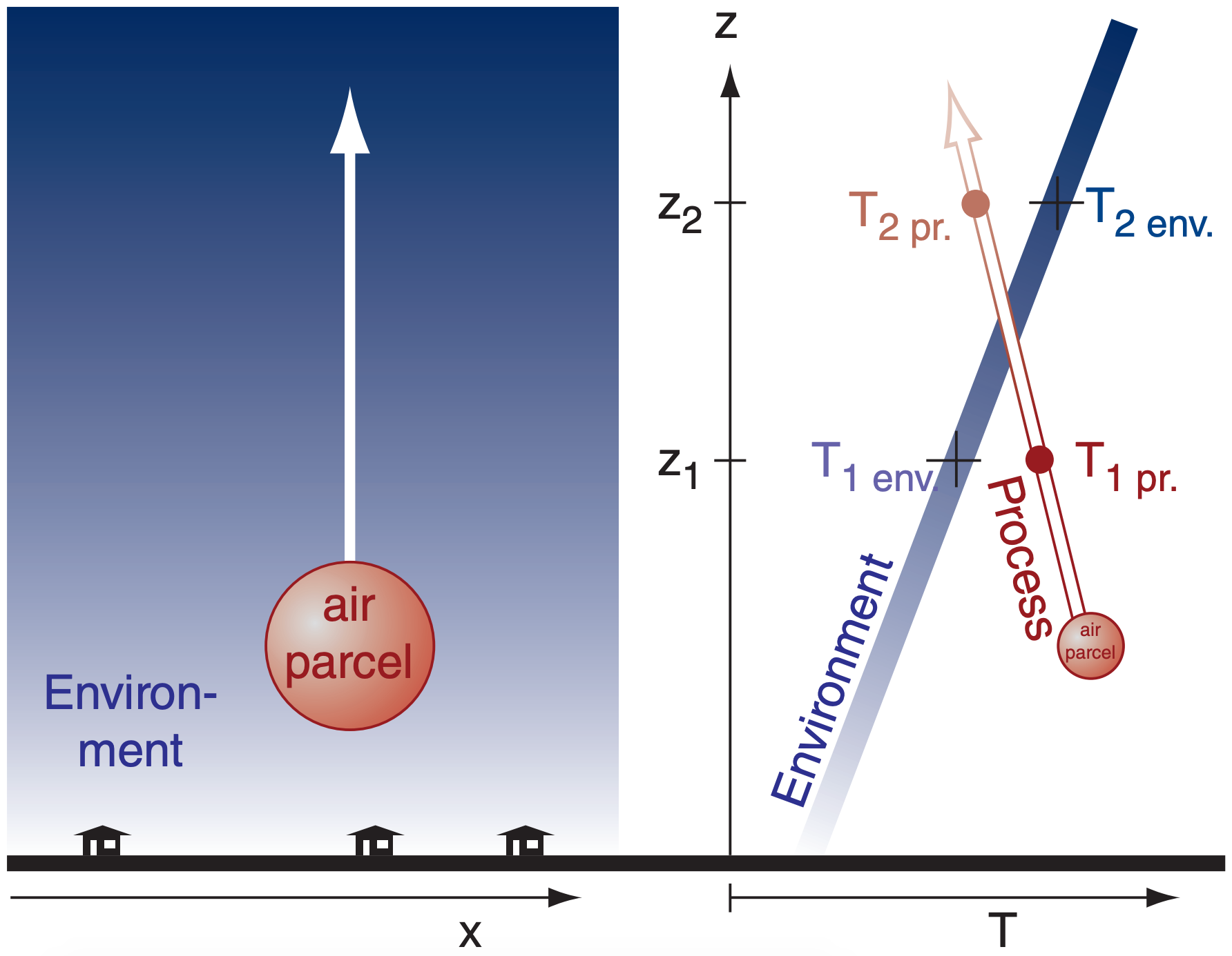
Outside the air parcel, assume the environmental air is relatively stationary. This is the ambient environment through which the air parcel moves. But this environment could have different temperatures at different altitudes, allowing us to define an environmental lapse rate (Figure 3.3). By sampling the ambient air at different heights using weather instruments such as radiosondes (weather balloons) and then plotting T vs. z as a graph, the result is an environmental sounding or vertical temperature profile of the environment. The environmental sounding changes as the weather evolves, but this is usually slow relative to parcel processes. Thus, the environment is often approximated as being unchanging (i.e., static).
The temperature difference (Figure 3.3) between the parcel and its environment is crucial for determining parcel buoyancy and storm development. This is our motivation for examining both lapse rates.
Sample Application
Find the lapse rate in the troposphere for a standard atmosphere.
Find the Answer
Given: Std. Atmos. Table 1-5 in Chapter 1, , where T= –56.5°C at z = 11 km, and T = +15°C at z = 0 km.
Find: Γ = ? °C km–1
Apply eq. (3.6): Γ = – (–56.5 – 15°C) / (11–0 km) = +6.5 °C km–1
Check: Positive Γ, because T decreases with z.
Exposition: This is the environmental lapse rate of the troposphere. It indicates a static background state.
3.4.3. Dry Adiabatic Lapse Rate
The word adiabatic means zero heat transfer (∆q = 0). For the protected inner core of air parcels, this means no thermal energy entering or leaving the air parcel from outside (Figure 3.2). Nonetheless, internal processes are allowed.
For the special case of humid air with no liquid water or ice carried with the parcel (and no water phase changes; hence, a “dry” process), eq. (3.5) gives:
\(\ \begin{align}\frac{\Delta T}{\Delta z}=-\left(\frac{|g|}{C_{p}}\right)=-9.8 \mathrm{Kkm}^{-1}\tag{3.7}\end{align}\)
Recalling that the lapse rate is the negative of the vertical temperature gradient, we can define a “dry” adiabatic lapse rate Γd as:
\(\ \begin{align}\Gamma_{d}=9.8 \mathrm{K} \mathrm{km}^{-1}=9.8^{\circ} \mathrm{C} \mathrm{km}^{-1}\tag{3.8}\end{align}\)
(Degrees K and °C are interchangeable in this equation for this process lapse rate, because they represent a temperature change with height.)
The HIGHER MATH box at left shows how this dry adiabatic lapse rate can be expressed as a function of pressure P:
\(\ \begin{align} \frac{\Delta T}{T}=\frac{\Re_{d}}{C_{p}} \cdot\left(\frac{\Delta P}{P}\right)\tag{3.9}\end{align}\)
or
\(\ \begin{align} \frac{T_{2}}{T_{1}}=\left(\frac{P_{2}}{P_{1}}\right)^{\Re_{d} / C_{p}}\tag{3.10}\end{align}\)
where ℜd/Cp = 0.28571 (dimensionless) for dry air, and where temperatures are in Kelvin.
Start with the First Law of Thermodynamics (eq. 3.2d), but written more precisely using virtual temperature Tv to account for arbitrary concentrations of water vapor in the air. Set ∆q = 0 because adiabatic means no heat transfer:
\(\mathrm{d} P=\rho \cdot C_{p} \cdot \mathrm{d} T_{v}\)
Use the ideal gas law ρ = P/(ℜd · Td ) to eliminate ρ:
\(\mathrm{d} P=\frac{P \cdot C_{p} \cdot \mathrm{d} T_{v}}{\Re_{d} \cdot T_{v}}\)
Group temperature & pressure terms on opposite sides of the eq.:
\(\frac{\mathrm{d} P}{P}=\frac{C_{p}}{\Re_{d}} \cdot \frac{\mathrm{d} T_{v}}{T_{v}}\)
Integrate from starting (P1, Tv1) to ending (P2, Tv2):
\(\int_{P_{1}}^{P_{2}} \frac{\mathrm{d} P}{P}=\frac{C_{p}}{\Re_{d}} \cdot \int_{T_{v 1}}^{T_{v 2}} \frac{\mathrm{d} T_{v}}{T_{v}}\)
assuming Cp/ℜd is somewhat constant. The integral is:
\(\left.\ln (P)\right|_{P_{1}} ^{P_{2}}=\left(C_{p} / \Re_{d}\right) \cdot \ln \left(T_{v}\right)_{T_{v 1}}^{T_{v 2}}\)
Insert limits of integration. Also: ln(a) –ln(b) = ln(a/b)
Thus:
\(\ln \left(\frac{P_{2}}{P_{1}}\right)=\left(C_{p} / \Re_{d}\right) \cdot \ln \left(\frac{T_{v 2}}{T_{v 1}}\right)\)
Multiply both sides by ℜd /Cp :
\(\left(\mathfrak{R}_{d} / C_{p}\right) \cdot \ln \left(\frac{P_{2}}{P_{1}}\right)=\ln \left(\frac{T_{v 2}}{T_{v 1}}\right)\)
Use the relationship: a·ln(b) = ln(ba):
\(\ln \left[\left(\frac{P_{2}}{P_{1}}\right)^{\Re_{d} / C_{p}}\right]=\ln \left(\frac{T_{v 2}}{T_{v 1}}\right)\)
The anti-log of the equation ( eLHS = eRHS ) yields:
\(\ \begin{align}\left(\frac{P_{2}}{P_{1}}\right)^{\Re_{d} / C_{p}}=\frac{T_{v 2}}{T_{v 1}}\tag{3.10}\end{align}\)
Sample Application
An air parcel with initial (z, P, T) = (100m, 100 kPa, 20°C) rises adiabatically to (z, P) = (1950 m, 80 kPa). Find its new T, & compare eqs. (3.7) & (3.10).
Find the Answer
Given: P1 = 100 kPa, P2 = 80 kPa, T1 = 20°C = 293K z1 = 100 m, z2 = 1950 m
Find: T2 = ? °C
First, apply eq. (3.7), which is a function of z:
T2 = T1 + (∆z)·(–Γd) = 20°C – (1950–100m)·(0.0098°C/m) = 20°C – 18.1°C = 1.9°C.
Compare with eq. (3.10), which is a function of P:
T2 = (293K) · [(80kPa)/(100kPa)]0.28571
T2 = 293K · 0.9382 = 274.9 K = 1.9°C
Check: Both equations give the same answer, so either equation would have been sufficient by itself.
3.4.4. Potential-temperature Definition
When an air parcel rises/sinks ”dry” adiabatically into regions of lower/higher pressure, its temperature changes due to work done by/on the parcel, even though no thermal energy has been removed/ added. Define a new temperature variable called the potential temperature θ that is proportional to the sensible heat contained in the parcel, but which is unaffected by work done by/on the parcel.
Namely, potential temperature is constant for an adiabatic process (i.e., ∆q = 0) such as air-parcel ascent. Thus, we can use it as a conserved variable. θ can increase/decrease when sensible heat is added/removed. Such diabatic (non-adiabatic) heat transfer processes include turbulent mixing, condensation, and radiative heating (i.e., ∆q ≠ 0).
Knowing the air temperature T at altitude z, you can calculate the value of potential temperature θ from:
\(\ \begin{align}\theta(z)=T(z)+\Gamma_{d} \cdot z\tag{3.11}\end{align}\)
The units (K or °C) of θ(z) are the same as the units of T(z). There is no standard for z, so some people use height above mean sea level (MSL), while others use height above local ground level (AGL).
If, instead, you know air temperature T at pressure-level P, then you can find the value of θ from:
\(\ \begin{align} \theta=T \cdot\left(\frac{P_{o}}{P}\right)^{\Re_{d} / C_{p}}\tag{3.12}\end{align}\)
where ℜd/Cp = 0.28571 (dimensionless) and where temperatures must be in Kelvin. A reference pressure of Po = 100 kPa is often used, although some people use the local surface pressure instead. In this book we will assume that the surface pressure equals the reference pressure of Po = 100 kPa and will use z = 0 at that surface, unless stated otherwise.
Both eqs. (3.11) and (3.12) show that θ = T at z = 0 or at P = Po. Thus θ is the actual temperature that an air parcel potentially has if lowered to the reference level adiabatically.
A virtual potential temperature θv for humid air having water-vapor mixing ratio r but containing no solid or liquid water is defined as:
\(\ \begin{align} \theta_{v}=\theta \cdot[1+(a \cdot r)]\tag{3.13}\end{align}\)
where a = 0.61 gair/gwater vapor . If the air contains ice crystals, cloud drops, or rain drops, then virtual potential temperature is given by:
\(\ \begin{align}\theta_{v}=\theta \cdot\left[1+(a \cdot r)-r_{L}-r_{I}\right]\tag{3.14}\end{align}\)
where rL is the liquid-water mixing ratio and rI = ice mixing ratio. Mixing ratio is described in the Water Vapor chapter; it is the ratio of grams of water per gram of air. The θ and θv values in the previous three equations must be in units of Kelvin.
An advantage of θv is that it can be used to calculate the buoyancy of air parcels that contain water — useful for anticipating storm characteristics. θv is constant only when there is no phase changes and no heat transfer; namely, no latent or sensible heat is absorbed or released.
For air that is rising within clouds, with water vapor condensing, it is usually the case that the air is saturated (= 100% relative humidity; see the Water Vapor chapter for details). As a result, the watervapor mixing ratio r can be replaced with rs , the saturation mixing ratio.
\(\ \begin{align} \theta_{v}=\theta \cdot\left[1+\left(a \cdot r_{s}\right)-r_{L}\right]\tag{3.15}\end{align}\)
where a = 0.61 gair/gwater vapor , as before.
However, there are other situations where the air is NOT saturated, but contains liquid water. An example is the non-cloudy air under a cloud base, through which rain is falling at its terminal velocity. For this case, eq (3.14) should be used with an unsaturated value of water-vapor mixing ratio. This situation occurs often, and can be responsible for damaging downbursts of air (see the Thunderstorm chapters).
Why use potential temperature? Because it makes it easier to compare the temperatures of air parcels at two different heights — important for determining if air will buoyantly rise to create thunderstorms. For example, suppose air parcel A has temperature TA = 20°C at z = 0, while air parcel B has TB = 15°C at z = 1 km. Parcel A is warmer than parcel B.
Does that mean that parcel A is buoyant (warmer and wants to rise) relative to parcel B? The answer is no, because when parcel B is moved dry adiabatically to the altitude of parcel A, then parcel B is 5°C warmer than parcel A due to adiabatic warming. In fact, you can move parcels A and B to any common altitude, and after considering their adiabatic warming or cooling, parcel B will always be 5°C warmer than parcel A.
The easiest way to summarize this effect is with potential temperature. Using eq. (3.11), we find that θA = 20°C and θB = 25°C approximately. θA and θB keep their values (because θ is a conserved variable) no matter to what common altitude you move them, thus θB is always 5 °C warmer than θA in this illustration.
Another application for potential temperature is to label lines on a thermodynamic diagram, such as described next.
3.4.5. Intro to Thermo Diagrams
Convection is a vertical circulation associated with “warm air rising” and “cold air sinking”. Meteorologists forecast the deep convection of thunderstorms and their hazards, or the shallow convection of thermals that disperse air pollutants.
The phrase “warm air rising” relates to the temperature difference ∆T between an air parcel and its surrounding environment. Air-parcel-temperature variation with altitude can be anticipated using heatand water-conservation relationships. However, the surrounding environmental temperature profile can have a somewhat arbitrary shape that can be measured by a sounding balloon, but which is not easily described by analytical equations. So it can be difficult to mathematically describe ∆T vs. altitude.
Instead, graphical solutions can be used to estimate buoyancy and convection. We call these graphs “thermodynamic diagrams”. In this book, I will abbreviate the name as “thermo diagram”.
The diagram is set up so that higher in the diagram corresponds to higher in the atmosphere. In the real atmosphere, pressure decreases approximately logarithmically with increasing altitude, so we often use pressure P along the y-axis as a surrogate for altitude. Along the x-axis is air temperature T. The thin green lines in Figure 3.4 show the (P, T) basis for a thermo diagram as a semi-log graph.
We can use eq. (3.10) to solve for the “dry” adiabatic temperature change experienced by rising air parcels. These are plotted as the thick orange diagonal lines in Figure 3.4 for a variety of starting temperatures at P = 100 kPa. These “dry adiabat” lines (also known as isentropes), are labeled with θ because potential temperature is conserved for adiabatic processes.
If you know the initial (P, T) of the air parcel, then plot it as a point on the thermo diagram. Move parallel to the orange lines to the final pressure altitude. At that final point, read down vertically to find the parcel’s final temperature.
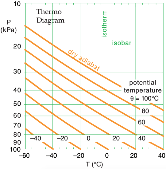
One of the advantages of thermo diagrams is that you do NOT need to calculate adiabatic temperature changes, because they are already calculated and plotted for you for a variety of different starting temperatures. If the starting temperature you need is not already plotted, you can mentally interpolate between the drawn lines as you raise or lower air parcels.
However, it is a useful exercise to see how such a thermo diagram can be created with a tool as simple as a computer spreadsheet.
The green (or dark-grey) items in the spreadsheet below were typed directly as numbers or words. You can follow along on your own spreadsheet. (You don’t need to use the same colors — black is OK.)
The orange (or light-grey) numbers were calculated by entering a formula (eq. 3.10) into the bottom leftmost orange cell, and then “filling up” and “filling right” that equation into the other orange cells. But before you fill up and right, be sure to use the dollar sign “$” as shown below. It holds the column ID constant if it appears in front of the ID letter, or holds the row constant if in front of the ID number. Here is the equation for the bottom left orange cell (B12): = ( (B$13+273) * ($A12/$A$13)^0.28571 ) - 273
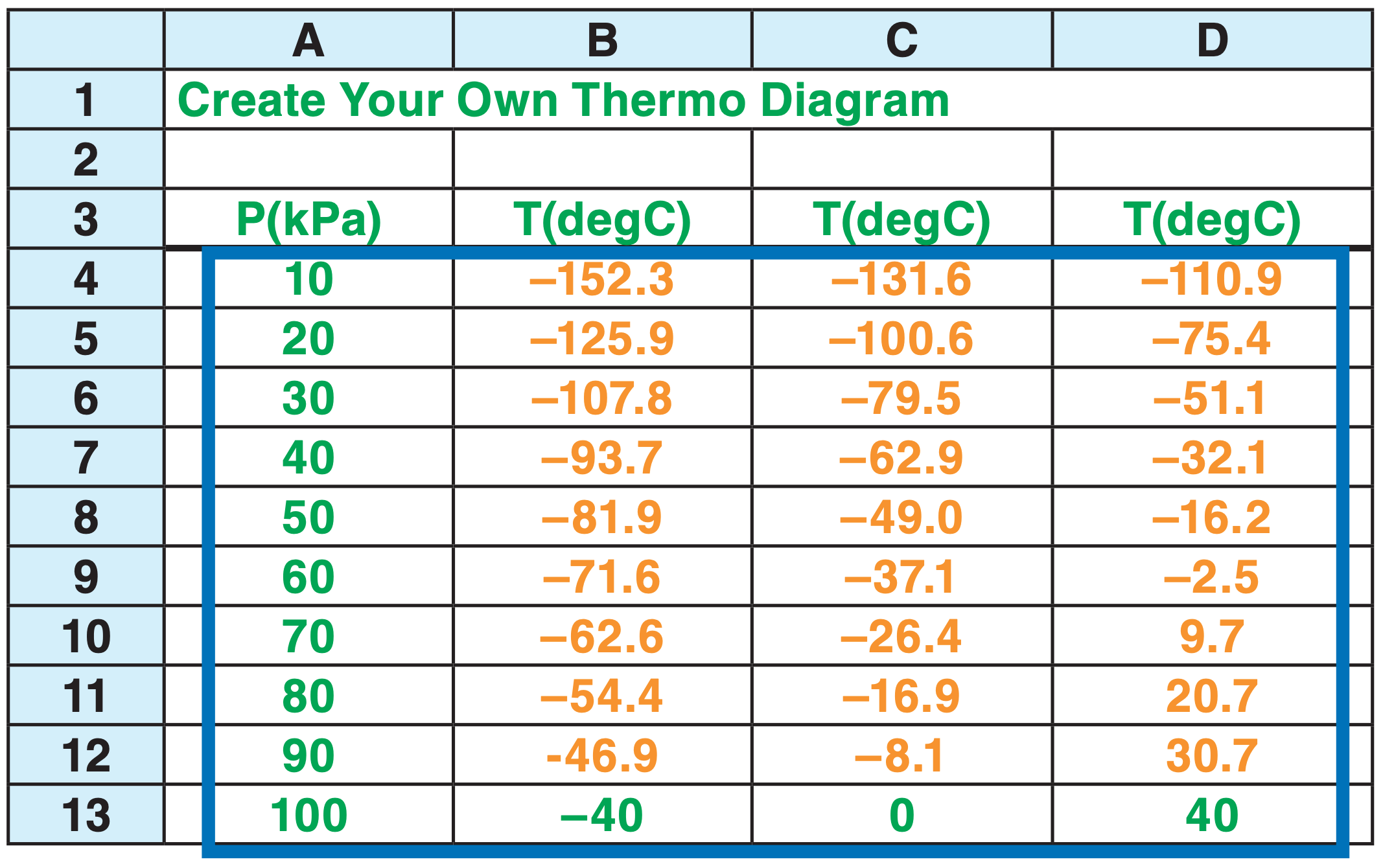
Different spreadsheet versions have different ways to create graphs. Select the cells that I outlined with the dark blue rectangle. Click on the Graph button, select the “XY scatter”, and then select the option that draws straight line segments without data points.
Under the Chart, Source Data menu, select Series. Then manually switch the columns for the X and Y data for each series — this does an axis switch. On the graph, click on the vertical axis to get the Format Axis dialog box, and select the Scale tab. Check the Logarithmic scale box, and the Values in Reverse Order box. A bit more tidying up will yield a graph with 3 curves similar to Figure 3.4. Try adding more curves.
Sample Application
Given air at P = 70 kPa with T = –1°C. Find θ using the thermo diagram of Figure 3.4.
Find the Answer
Given: P = 70 kPa , T = –1°C
Find: θ = ? °C
First, use the thermo diagram to find where the 70 kPa isobar and the –1°C isotherm intersect. (Since the –1°C isotherm wasn’t drawn on this diagram, we must mentally interpolate between the lines that are drawn.) The adiabat that passes through this intersection point indicates the potential temperature (again, we must interpolate between the adiabats that are drawn). By extending this adiabat down to the reference pressure of 100 kPa, we can read off the temperature 28°C, which corresponds to a potential temperature of θ = 28°C .
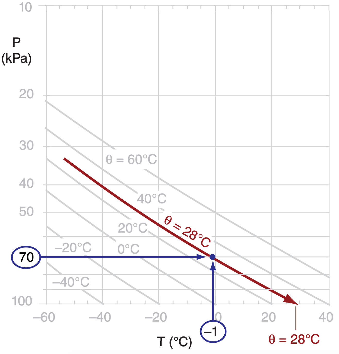
Check: Physics and units are reasonable.
Exposition: This exercise is the same as part (a) of the previous exercise, for which we calculated θ = 301 K = 28°C. Yes, the answers agree.
The advantage of using an existing printed thermo diagram is that we can draw a few lines and quickly find the answer without doing any calculations. So it can make our lives easier, once we learn how to use it.


