2.2: Radiation Principles

2.3.1. Propagation

Radiation can be modeled as electromagnetic waves or as photons. Radiation propagates through a vacuum at a constant speed: co = 299,792,458 m·s^–1. For practical purposes, you can approximate this speed of light as c_o ≈ 3x108 m·s^–1. Light travels slightly slower through air, at roughly c = 299,710,000 m·s^–1 at standard sea-level pressure and temperature, but the speed varies slightly with thermodynamic state of the air (see the Optics chapter).

Using the wave model of radiation, the wavelength λ (m·cycle^–1) is related to the frequency, ν (Hz = cycles·s^–1) by:

\(\ \begin{align} \lambda \cdot v=c_{o}\tag{2.12}\end{align}\)

Wavelength units are sometimes abbreviated as (m). Because the wavelengths of light are so short, they are often expressed in units of micrometers (µm).

Wavenumber is the number of waves per meter: σ (cycles·m–1) = 1/λ. An alternative wavenumber definition is radians per meter (= 2π/λ). Their units are sometimes abbreviated as (m^–1). Circular frequency or angular frequency is ω (radians s^–1) = 2π·ν. Its units are sometimes abbreviated as (s^–1).

Sample Application

Red light has a wavelength of 0.7 µm. Find its frequency, circular frequency, and wavenumber in a vacuum.

Find the Answer

Given: c_o = 299,792,458 m s^–1, λ = 0.7 µm

Find: ν = ? Hz, ω = ? s^–1 , σ = ? m^–1 .

Use eq. (2.12), solving for ν:

ν = c_o/λ = (3x10⁸ m s^–1) / (0.7x10^–6 m cycle^–1) = 4.28x10¹⁴ Hz.

ω = 2π·ν = 2·(3.14159)·(4.28x10¹⁴ Hz) = 2.69x10¹⁵ s^–1.

σ = 1/λ = 1 / (0.7x10^–6 m cycle^–1) = 1.43x10⁶ m^–1.

Check: Units OK. Physics reasonable

Exposition: Wavelength, wavenumber, frequency, and circular frequency are all equivalent ways to express the “color” of radiation.

2.3.2. Emission

Objects warmer than absolute zero can emit radiation. An object that emits the maximum possible radiation for its temperature is called a blackbody. Planck’s law gives the amount of blackbody monochromatic (single wavelength or color) radiant flux leaving an area, called emittance or radiant exitance, E_λ*:

\(\ \begin{align}E_{\lambda}^{*}=\dfrac{c_{1}}{\lambda^{5} \cdot\left[\exp \left(c_{2} /(\lambda \cdot T)\right)-1\right]}\tag{2.13}\end{align}\)

where T is absolute temperature, and the asterisk indicates blackbody. The two constants are:

c₁ = 3.74 x 10⁸ W·m^–2 · µm⁴ , and

c₂ = 1.44 x 10⁴ µm·K.

Eq. (2.13) and constant c1 already include all directions of exiting radiation from the area. E_λ* has units of W·m^-2 µm^–1 ; namely, flux per unit wavelength. For radiation approaching an area rather than leaving it, the radiant flux is called irradiance.

The ideal gas law is easy to remember and apply in solving problems, as long as you get the proper values a

Figure 2.8 Planck radiant exitance, E_λ*, from a blackbody approximately the same temperature as the sun.

Figure 2.9 Planck radiant exitance, E_λ*, from a blackbody approximately the same temperature as the Earth.

Actual objects can emit less than the theoretical blackbody value: E_λ = e_λ·E_λ* , where 0 ≤ e_λ ≤ 1 is emissivity, a measure of emission efficiency.

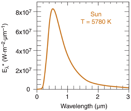
The Planck curve (eq. 2.13) for emission from a blackbody the same temperature as the sun (T = 5780 K) is plotted in Figure 2.8. Peak emissions from the sun are in the visible range of wavelengths (0.38 – 0.74 µm, see Table 2-3). Radiation from the sun is called solar radiation or short-wave radiation.

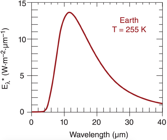
The Planck curve for emission from a blackbody that is approximately the same temperature as the whole Earth-atmosphere system (T ≈ 255 K) is plotted in Figure 2.9. Peak emissions from this idealized average Earth system are in the infrared range 8 to 18 µm. This radiation is called terrestrial radiation, long-wave radiation, or infrared (IR) radiation.

The wavelength of the peak emission is given by Wien’s law:

\(\ \begin{align} \lambda_{\max }=\dfrac{a}{T}\tag{2.14}\end{align}\)

where a = 2897 µm·K.

The total amount of emission (= area under Planck curve = total emittance) is given by the Stefan-Boltzmann law:

\(\ \begin{align}E^{*}=\sigma_{S B} \cdot T^{4}\tag{2.15}\end{align}\)

where σ_SB = 5.67x10^–8 W·m^–2·K^–4 is the StefanBoltzmann constant, and E* has units of W·m^–2. More details about radiation emission are in the Satellites & Radar chapter in the sections on weather satellites.

Table 2-3. Ranges of wavelengths λ of visible colors. Approximate center wavelength is in boldface. For more info, see Chapter 22 on Atmospheric Optics.
Color	λ (µm)
Red	0.625 - 0.650 - 0.740
Orange	0.590 - 0.600 - 0.625
Yellow	0.565 - 0.577 - 0.590
Green	0.500 - 0.510 - 0.565
Cyan	0.485 - 0.490 - 0.500
Blue	0.460 - 0.475 - 0.485
Indigo	0.425 - 0.445 - 0.460
Violet	0.380 - 0.400 - 0.425

Sample Application

What is the total radiant exitance (radiative flux) emitted from a blackbody Earth at T = 255 K, and what is the wavelength of peak emission?

Find the Answer

Given: T = 255 K

Find: E* = ? W·m–2 , λ_max = ? µm

Sketch:

Use eq. (2.15):

E*= (5.67x10^–8 W·m^–2·K^–4)·(255 K)⁴ = 240 W·m^–2

Use eq. (2.14):

λ_max = (2897 µm·K) / (255 K) = 11.36 µm

Check: Units OK. λ agrees with peak in Figure 2.9.

Exposition: You could create the same flux by placing a perfectly-efficient 240 W light bulb in front of a parabolic mirror that reflects the light and IR radiation into a beam that is 1.13 m in diameter.

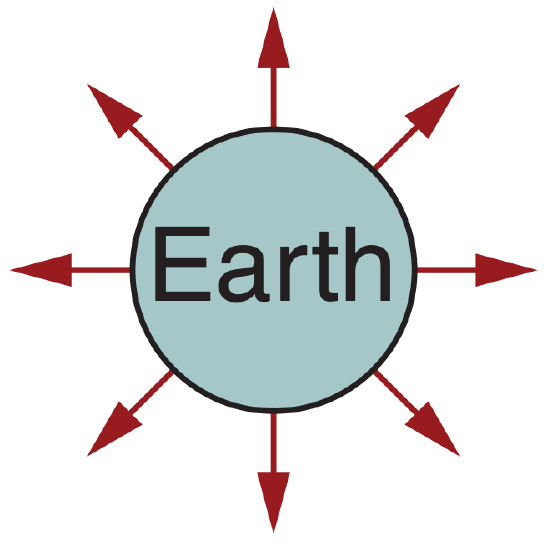
For comparison, the surface area of the Earth is about 5.1x10¹⁴ m², which when multiplied by the flux gives the total emission of 1.22x10¹⁷ W. Thus, the Earth acts like a large-wattage IR light bulb.

HIGHER MATH • Incremental Changes

What happens to the total radiative exitance given by eq. (2.15) if temperature increases by 1°C? Such a question is important for climate change.

Find the Answer using calculus:

Calculus allows a simple, elegant way to find the solution. First, expand eq. (1.15) into a Taylor’s series:

E* (T + ΔT) = E* (T)+ ΔT·E*′(T)+!

E* (T +∆ T )− E* (T ) = ∆ T ·4·σ_SB ·T 3 +!

ΔE* ≈ ΔT·4·σ_SB·T3

Thus, a fixed increase in temperature of ∆T = 1°C causes a much larger radiative exitance increase at high temperatures than at cold, because of the T³ factor on the right side of the equation.

Find the Answer using algebra:

This particular problem could also have been solved using algebra, but with a more tedious and less elegant solution. First let

E₂ = σ_SB ^. T₂⁴ and E₁ = σ_SB ^. T₁⁴

Next, take the difference between these two eqs:

∆E = E₂ - E₁ = σ ^. [T₂⁴ - T₁⁴]

Recall from algebra that (a² – b²) = (a – b)·(a + b)

\(\Delta E=\sigma_{S B} \cdot\left(T_{2}^{2}-T_{1}^{2}\right) \cdot\left(T_{2}^{2}+T_{1}^{2}\right)\)

\(\Delta E=\sigma_{S B} \cdot\left(T_{2}-T_{1}\right) \cdot\left(T_{2}+T_{1}\right) \cdot\left(T_{2}^{2}+T_{1}^{2}\right)\)

Since (T₂ – T₁) / T₁ << 1, then (T₂ – T₁ ) = ∆T, but T₂ + T₁ ≈ 2T, and T₂² + T₁² ≈ 2·T². This gives:

∆E = σ_SB ^. ∆T ^. 2T ^. 2T²

or

∆E ≈ σ_{SB .} [4T³∆T]

which is identical to the answer from calculus.

We were lucky this time, but it is not always possible to use algebra where calculus is needed.

A SCIENTIFIC PERSPECTIVE • Scientific Laws – The Myth

There are no scientific laws. Some theories or models have succeeded for every case tested so far, yet they may fail for other situations. Newton’s “Laws of Motion” were accepted as laws for centuries, until they were found to fail in quantum mechanical, relativistic, and galaxy-size situations. It is better to use the word “relationship” instead of “law”. In this textbook, the word “law” is used for sake of tradition.

Einstein said “No amount of experimentation can ever prove me right; a single experiment can prove me wrong.”

Because a single experiment can prove a relationship wrong, it behooves us as scientists to test theories and equations not only for reasonable values of variables, but also in the limit of extreme values, such as when the variables approach zero or infinity. These are often the most stringent tests of a relationship.

Example

Query: The following is an approximation to Planck’s law.

\(\ \begin{align}E_{\lambda}^{*}=c_{1} \cdot \lambda^{-5} \cdot \exp \left[-c_{2} /(\lambda \cdot T)\right]\tag{a}\end{align}\)

Why is it not a perfect substitute?

Find the Answer If you compare the numerical answers from eqs. (2.13) and (a), you find that they agree very closely over the range of temperatures of the sun and the Earth, and over a wide range of wavelengths. But...

a) What happens as temperature approaches absolute zero? For eq. (2.13), T is in the denominator of the argument of an exponential, which itself is in the denominator of eq. (2.13). If T = 0, then 1/T = ∞ . Exp(∞) = ∞ , and 1/∞ = 0. Thus, E_λ* = 0, as it should. Namely, no radiation is emitted at absolute zero (according to classical theory).

For eq. (a), if T = 0, then 1/T = ∞ , and exp(–∞) = 0. So it also agrees in the limit of absolute zero. Thus, both equations give the expected answer.

b) What happens as temperature approaches infinity? For eq. (2.13), if T = ∞ , then 1/T = 0 , and exp(0) = 1. Then 1 – 1 = 0 in the denominator, and 1/0 = ∞ . Thus, E_λ* = ∞, as it should. Namely, infinite radiation is emitted at infinite temperature.

For eq. (a), if T = ∞ , then 1/T = 0 , and exp(–0) = 1. Thus, E_λ* = c₁ · λ^–5 , which is not infinity. Hence, this approaches the wrong answer in the ∞ T limit.

Conclusion: Eq. (a) is not a perfect relationship, because it fails for this one case. But otherwise it is a good approximation over a wide range of normal temperatures.

2.3.3. Distribution

Radiation emitted from a spherical source decreases with the square of the distance from the center of the sphere:

\(\ \begin{align}E_{2}=E_{1}^{*} \cdot\left(\dfrac{R_{1}}{R_{2}}\right)^{2}\tag{2.16}\end{align}\)

where R is the radius from the center of the sphere, and the subscripts denote two different distances from the center. This is called the inverse square law.

The reasoning behind eq. (2.16) is that as radiation from a small sphere spreads out radially, it passes through ever-larger conceptual spheres. If no energy is lost during propagation, then the total energy passing across the surface of each sphere must be conserved. Because the surface areas of the spheres increase with the square of the radius, this implies that the energy flux density must decrease at the same rate; i.e., inversely to the square of the radius.

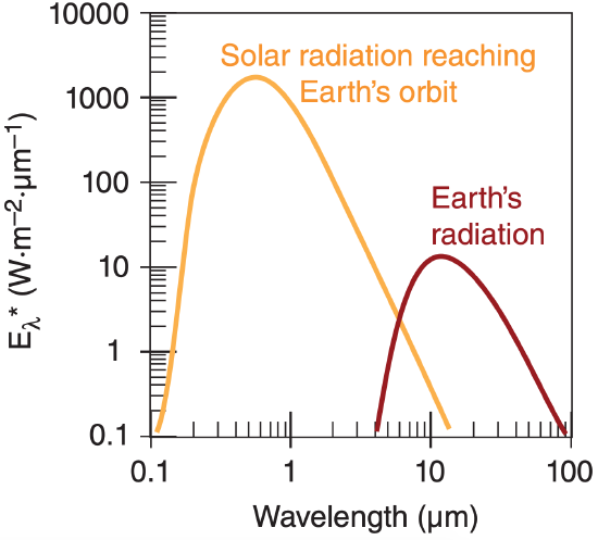
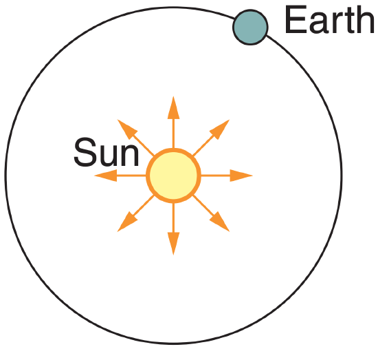
From eq. (2.16) we expect that the radiative flux reaching the Earth’s orbit is greatly reduced from that at the surface of the sun. The solar emissions of Figure 2.8 must be reduced by a factor of 2.167x10^–5, based on the square of the ratio of solar radius to Earth-orbital radius from eq. (2.16). This result is compared to the emission from Earth in Figure 2.10.

The area under the solar-radiation curve in Figure 2.10 is the total (all wavelengths) solar irradiance (TSI), S₀, reaching the Earth’s orbit. We call it an irradiance here, instead of an emittance, because relative to the Earth it is an incoming radiant flux. This quantity was formerly called the solar constant but we now know that it varies slightly. The average value of solar irradiance measured at the Earth’s orbit by satellites for a quiet sun (during sunspot minima) is about

\(\ \begin{align}S_{o}=1361 \mathrm{W} \cdot \mathrm{m}^{-2}\tag{2.17}\end{align}\)

In kinematic units (based on sea-level density), the solar irradiance is roughly S_o = 1.11 K·m s^–1.

During the 11-year sunspot cycle the solar irradiance normally increases by about 1.4 W·m^–2 during sunspot maxima. One example of a longer term variation in solar activity is the Maunder Minimum in the late 1600s, during which the solar irradiance was perhaps 2.7 to 3.7 W·m^–2 less than values during modern solar minima. Such irradiance changes could cause subtle changes (0.3 to 0.4°C) in global climate. See the Climate chapter for more info on solar variability.

Figure 2.10 Blackbody radiance E* reaching top of Earth’s atmosphere from the sun and radiance of terrestrial radiation leaving the top of the atmosphere, plotted on a log-log graph.

Sample Application

Estimate the value of the solar irradiance reaching the orbit of the Earth, given a sun surface temperature (5770 K), sun radius (6.96x10⁵ km), and orbital radius (1.495x10⁸ km) of the Earth from the sun.

Find the Answer

Given: T_sun = 5770 K

R_sun = 6.96x105 km = solar radius

R_Earth = 1.495x108 km = Earth orbit radius

Find: S_o = ? W·m^–2

Sketch:

First, use eq. (2.15):

E₁* = (5.67x10^–8 W·m^–2·K^–4)·(5770 K)⁴ = 6.285x10⁷ W·m^–2.

Next, use eq. (2.16), with R₁ = R_sun & R₂ = R_Earth So = E₂*=(6.285x10⁷ W·m^–2)·(6.96x10⁵ km/1.495x10⁸ km)² = 1362 W·m^–2.

Check: Units OK, Sketch OK. Physics OK.

Exposition: Answer is nearly equal to that measured by satellites, as given in eq. (2.17).

According to the inverse-square law, variations of distance between Earth and sun cause changes of the solar radiative forcing, S, that reaches the top of the atmosphere:

\(\ \begin{align}S=S_{O} \cdot\left(\dfrac{\bar{R}}{R}\right)^{2}\tag{2.18}\end{align}\)

where S_o = 1361 W·m^–2 is the average total solar irradiance measured at an average distance \(\ \bar{R}\) = 149.6 Gm between the sun and Earth, and R is the actual distance between Earth and the sun as given by eq. (2.4). Remember that the solar irradiance and the solar radiative forcing are the fluxes across a surface that is perpendicular to the solar beam, measured above the Earth’s atmosphere.

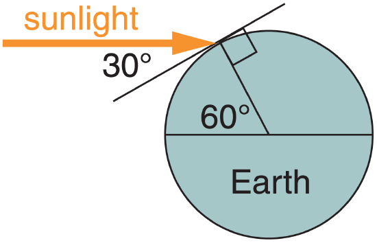
Let irradiance E be any radiative flux crossing a unit area that is perpendicular to the path of the radiation. If this radiation strikes a surface that is not perpendicular to the radiation, then the radiation per unit surface area is reduced according to the sine law. The resulting flux, F_rad, at this surface is:

\(\ \begin{align}\mathbb{F}_{r a d}=E \cdot \sin (\Psi)\tag{2.19}\end{align}\)

where Ψ is the elevation angle (the angle of the sun above the surface). In kinematic form, this is

\(\ \begin{align}F_{r a d}=\dfrac{E}{\rho \cdot C_{p}} \cdot \sin (\Psi)\tag{2.20}\end{align}\)

where ρ·C_p is given under eq. (2.11).

Sample Application(§)

Using the results from an earlier Sample Application that calculated the true anomaly and sun-Earth distance for several days during the year, find the solar radiative forcing for those days.

Find the Answer

Given: R values from previously Sample Application Find: S = ? W·m^–2

Sketch: (same as Fig 2.2)

Use eq. (2.18).

Date	d	R(ν) (Gm)	S (W/m^2)
4 Jan	4	146.96	1418
18 Jan	18	147.04	1416
1 Feb	32	147.25	1412
15 Feb	46	147.60	1405
1 Mar	60	148.06	1397
15 Mar	74	148.60	1386
29 Mar	88	149.18	1376
12 Apr	102	149.78	1365
26 Apr	116	150.36	1354
21 Jun	172	151.88	1327
23 Sep	266	150.01	1361
22 Dec	356	147.03	1416

Check: Units OK. Physics OK.

Exposition: During N. Hemisphere winter, solar radiative forcing is up to 50 W·m^–2 larger than average.

Sample Application

During the equinox at noon at latitude ϕ =60°, the solar elevation angle is Ψ = 90° – 60° = 30°. If the atmosphere is perfectly transparent, then how much radiative flux is absorbed into a perfectly black asphalt parking lot?

Find the Answer

Given: Ψ = 30° = elevation angle E = S_o = 1361 W·m^–2. solar irradiance

Find: Frad = ? W·m^–2

Sketch:

Use eq. (2.19):

F_rad = (1361 W·m^–2)·sin(30°) = 680.5 W·m^–2.

Check: Units OK. Sketch OK. Physics OK.

Exposition: Because the solar radiation is striking the parking lot at an angle, the radiative flux into the parking lot is half of the solar irradiance.

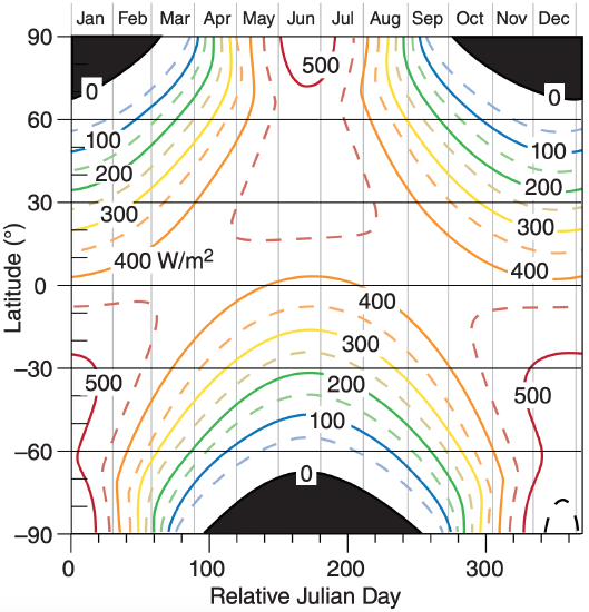
2.3.4. Average Daily Insolation

The contraction “insolation” means “incoming solar radiation” at the top of the atmosphere. The average daily insolation \(\ \bar{E}\) takes into account both the solar elevation angle (which varies with season and time of day) and the duration of daylight. For example, there is more total insolation at the poles in summer than at the equator, because the low sun angle near the poles is more than compensated by the long periods of daylight.

\(\begin{align} \bar{E}=\dfrac{S_{O}}{\pi} \cdot\left(\dfrac{a}{R}\right)^{2} \cdot\left[h_{O}^{\prime} \cdot \sin (\phi) \cdot \sin \left(\delta_{S}\right)+\right.\left.\cos (\phi) \cdot \cos \left(\delta_{S}\right) \cdot \sin \left(h_{O}\right)\right]\tag{2.21} \end{align}\)

where S_o =1361 W m^–2 is the solar irradiance, a = 149.457 Gm is Earth’s semi-major axis length, R is the actual distance for any day of the year, from eq. (2.4), and ϕ = latitude. In eq. (2.21), h_o’ is the sunset and sunrise hour angle in radians.

The hour angle h_o at sunrise and sunset can be found using the following steps:

\(\ \begin{align}\alpha=-\tan (\phi) \cdot \tan \left(\delta_{s}\right)\tag{2.22a}\end{align}\)

\(\ \begin{align}\beta=\min [1,(\max (-1, \alpha)]\tag{2.22b}\end{align}\)

\(\ \begin{align}h_{O}=\arccos (\beta)\tag{2.22c}\end{align}\)

Eq. (2.22b) truncates the argument of the arccos to be between –1 and 1, in order to account for high latitudes where there are certain days when the sun never sets, and other days when it never rises.

[CAUTION. When finding the arccos, your answer might be in degrees or radians, depending on your calculator, spreadsheet, or computer program. Determine the units by experimenting first with the arccos(0), which will either give 90° or π/2 radians. If necessary, convert the hour angle to units of radians, the result of which is h_o’.]

Figure 2.11 shows the average incoming solar radiation vs. latitude and day of the year, found using eq. (2.21). For any one hemisphere, \(\ \bar{E}\) has greater difference between equator and pole during winter than during summer. This causes stronger winds and more active extratropical cyclones in the winter hemisphere than in the summer hemisphere.

Figure 2.11 Average daily insolation \(\ \bar{E}\) (W m^–2) over the globe.

Sample Application

Find the average daily insolation over Vancouver during the summer solstice.

Find the Answer

Given: d = d_r = 173 at the solstice, ϕ = 49.25°N, λ_e = 123.1°W for Vancouver.

Find: \(\ \bar{E}\) = ? W m^–2

Use eq. (2.5): δ_s = Φ_r = 23.45°

Use eq. (2.2): M = 167.55°, and assume ν ≈ M.

Use eq. (2.4): R = 151.892 Gm.

Use eq. (2.22):

h_o = arccos[–tan(49.25°)·tan(23.45°)] = 120.23°

h_o’ = h_o·2π/360° = 2.098 radians

Use eq. (2.21):

\(\begin{aligned} \bar{E}=& \dfrac{\left(1361 \mathrm{W} \cdot \mathrm{m}^{-2}\right)}{\pi} \cdot\left(\dfrac{149 \mathrm{Gm}}{151.892 \mathrm{Gm}}\right)^{2} \cdot \left[2.098 \cdot \sin \left(49.25^{\circ}\right) \cdot \sin \left(23.45^{\circ}\right)+\right.\left.\cos \left(49.25^{\circ}\right) \cdot \cos \left(23.45^{\circ}\right) \cdot \sin \left(120.23^{\circ}\right)\right] \end{aligned}\)

\(\ \bar{E}\) = (1320 W m^–2)·[2.098(0.3016)+0.5174] = 483.5 Wm^–2

Check: Units OK. Physics OK. Agrees with Figure 2.11.

Exposition: At the equator on this same day, the average daily insolation is less than 400 Wm^–2 .

2.3.5. Absorption, Reflection & Transmission

The emissivity, e_λ, is the fraction of blackbody radiation that is actually emitted (see Table 2-4) at any wavelength λ. The absorptivity, a_λ, is the fraction of radiation striking a surface of an object that is absorbed (i.e., stays in the object as a different form of energy). Kirchhoff’s law states that the absorptivity equals the emissivity of a substance at each wavelength, λ. Thus,

\(\ \begin{align}a_{\lambda}=e_{\lambda}\tag{2.23}\end{align}\)

Some substances such as dark glass are semitransparent (i.e., some radiation passes through). A fraction of the incoming (incident) radiation might also be reflected (bounced back), and another portion might be absorbed. Thus, you can define the efficiencies of reflection, absorption, and transmission as:

\(\ \begin{align}r_{\lambda}=\dfrac{E_{\lambda} \text {reftected}}{E_{\lambda} \text { incident }}= reflectivity \tag{2.24}\end{align}\)

\(\ \begin{align}a_{\lambda}=\dfrac{E_{\lambda} \text {absorbed}}{E_{\lambda} \text {incident}}= absorptivity \tag{2.25}\end{align}\)

\(\ \begin{align}t_{\lambda}=\dfrac{E_{\lambda} \text {transmitted}}{E_{\lambda} \text {incident}}= transmissivity\tag{2.26}\end{align}\)

Values of e_λ, a_λ, r_λ, and t_λ are between 0 and 1.

The sum of the last three fractions must total 1, as 100% of the radiation at any wavelength must be accounted for:

\(\ \begin{align}1=a_{\lambda}+r_{\lambda}+t_{\lambda}\tag{2.27}\end{align}\)

or

\(\ \begin{align}E_{\lambda \text { incoming }}=E_{\lambda \text { absorbed }}+E_{\lambda \text { reflected }}+E_{\lambda \text { transmitted }}\tag{2.28}\end{align}\)

For opaque (t_λ = 0) substances such as the Earth’s surface, you find: a_λ = 1 – r_λ.

The reflectivity, absorptivity, and transmissivity usually vary with wavelength. For example, clean snow reflects about 90% of incoming solar radiation, but reflects almost 0% of IR radiation. Thus, snow is “white” in visible light, and “black” in IR. Such behavior is crucial to surface temperature forecasts.

Instead of considering a single wavelength, it is also possible to examine the net effect over a range of wavelengths. The ratio of total reflected to total incoming solar radiation (i.e., averaged over all solar wavelengths) is called the albedo, A :

\(\ \begin{align}A=\dfrac{E_{\text {reflected}}}{E_{\text {incoming}}}\tag{2.29}\end{align}\)

The average global albedo for solar radiation reflected from Earth is A = 30% (see the Climate chapter). The actual global albedo at any instant varies with ice cover, snow cover, cloud cover, soil moisture, topography, and vegetation (Table 2-5). The Moon’s albedo is only 7%.

The surface of the Earth (land and sea) is a very strong absorber and emitter of radiation.

Within the air, however, the process is a bit more complicated. One approach is to treat the whole atmospheric thickness as a single object. Namely, you can compare the radiation at the top versus bottom of the atmosphere to examine the total emissivity, absorptivity, and reflectivity of the whole atmosphere. Over some wavelengths called windows there is little absorption, allowing the radiation to “shine” through. In other wavelength ranges there is partial or total absorption. Thus, the atmosphere acts as a filter. Atmospheric windows and transmissivity are discussed in detail in the Satellites & Radar and Climate chapters.

Table 2-4. Typical infrared emissivities.
Surface	e	Surface	e
alfalfa	alfalfa	iron, galvan.	0.13-0.28
aluminum	0.01-0.05	leaf 0.8 µm	0.05-0.53
asphalt	0.95	leaf 1 µm	0.05-0.6
bricks, red	0.92	leaf 2.4 µm	0.7-0.97
cloud, cirrus	0.3	leaf 10 µm	0.97-0.98
cloud, alto	0.9	lumber, oak	0.9
cloud, low	1.0	paper	0.89-0.95
concrete	0.71-0.9	plaster, white	0.91
desert	0.84-0.91	sand, wet	0.98
forest, conif.	0.97	sandstone	0.98
forest, decid.	0.95	shrubs	0.9
glass	0.87-0.94	silver	0.02
grass	0.9-0.95	snow, fresh	0.99
grass lawn	0.97	snow, old	0.82
gravel	0.92	soils	0.9-0.98
human skin	0.95	soil, peat	0.97-0.98
ice	0.96	urban	0.85-0.95

Sample Application

If 500 W m^–2 of visible light strikes a translucent object that allows 100 W m^–2 to shine through and 150 W m^–2 to bounce off, find the transmissivity, reflectivity, absorptivity, and emissivity.

Find the Answer

Given: E_{λ incoming} = 500 W m^–2 , E_{λ transmitted} = 100 W m^–2 , E_{λ reflected} = 150 W m^–2

Find: a_λ = ? , e_λ = ? , r_λ = ? , and t_λ = ?

Use eq. (2.26): t_λ = (100 W m^–2) / (500 W m^–2) = 0.2

Use eq. (2.24): r_λ = (150 W m^–2) / (500 W m^–2) = 0.3

Use eq. (2.27): a_λ = 1 – 0.2 – 0.3 = 0.5

Use eq. (2.23): e_λ = a_λ = 0.5

Check: Units dimensionless. Physics reasonable.

Exposition: By definition, translucent means partly transparent, and partly absorbing.

Table 2-5. Typical albedos (%) for sunlight
Surface	A (%)	Surface	A (%)
alfalfa	23-32	forest, decid.	10-25
buildings	9	granite	12-18
clay, wet	16	grass, green	26
clay, dry	23	gypsum	55
cloud, thick	70-95	ice, gray	60
cloud, thin	20-65	lava	10
concrete	15-37	lime	45
corn	18	loam, wet	16
cotton	20-22	loam, dry	23
field, fallow	5-12	meadow, green	10-20
forest, conif.	5-15	potatoes	19
rice paddy	12	soil, red	17
road, asphalt	5-15	soil, sandy	20-25
road, dirt	18-35	sorghum	20
rye winter	18-23	steppe	20
sand dune	20-45	stones	20-30
savanna	15	sugar cane	15
snow, fresh	75-95	tobacco	19
snow, old	35-70	tundra	15-20
soil, dark wet	6-8	urban, mean	15
soil, light dry	16-18	water, deep	5-20
soil, peat	5-15	wheat	10-23

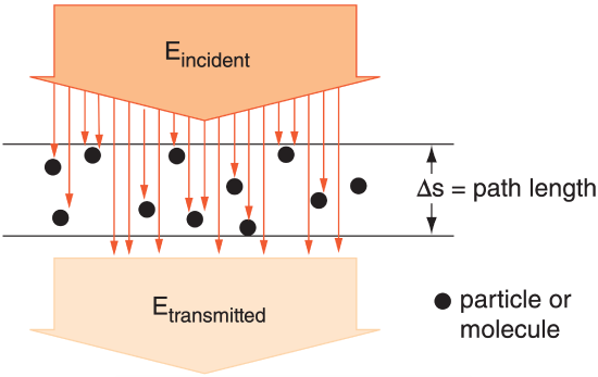
2.3.6. Beer’s Law

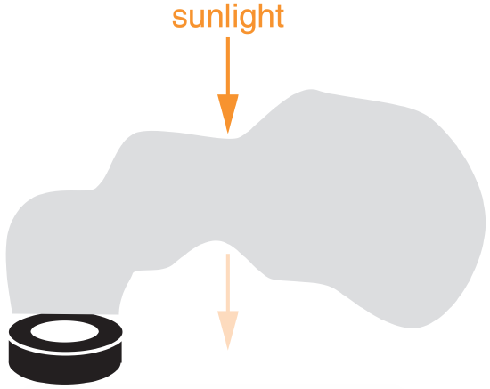
Sometimes you must examine radiative extinction (reduction of radiative flux) of radiation in a direct beam across a short path length ∆s within the atmosphere (Figure 2.12). Let n be the number density of radiatively important particles in the air (particles m^–3), and b be the extinction cross section of each particle (m² particle^–1), where this latter quantity gives the area of the shadow cast by each particle.

Figure 2.12 Reduction of radiation across an air path due to absorption and scattering by particles such as air-pollution aerosols or cloud droplets, illustrating Beer’s law.

Extinction can be caused by absorption and scattering of radiation. If the change in radiation is due only to absorption, then the absorptivity across this layer for a narrow beam of photons is

\(\ \begin{align}a=\dfrac{E_{\text {incident}}-E_{\text {transmitted}}}{E_{\text {incident}}}\tag{2.30}\end{align}\)

Beer’s law gives the relationship between incident radiative flux, Eincident, and transmitted radiative flux, Etransmitted, for a direct beam as

\(\ \begin{align}E_{\text {transmitted}}=E_{\text {incident}} \cdot \mathrm{e}^{-n \cdot b \cdot \Delta s}\tag{2.31a}\end{align}\)

Beer’s law can be written using an extinction coefficient, k:

\(\ \begin{align}E_{\text {transmitted}}=E_{\text {incident}} \cdot \mathrm{e}^{-k \cdot \rho \cdot \Delta s}\tag{2.31b}\end{align}\)

where ρ is the density of air, and k has units of m² g_air^–1 . The total extinction integrated across the whole path can be quantified by a dimensionless optical thickness (or optical depth in the vertical), \(\ \tau\), allowing Beer’s law to be rewritten as:

\(\ \begin{align}E_{\text {transmitted}}=E_{\text {incident}} \cdot e^{-\tau}\tag{2.31c}\end{align}\)

To simplify these equations, sometimes a volume extinction coefficient \(\ \gamma\) is defined by

\(\ \begin{align}\gamma=n \cdot b=k \cdot \rho\tag{2.32}\end{align}\)

Visual range (V, one definition of visibility) is the distance where the intensity of transmitted light has decreased to 2% of the incident light. It estimates the max distance ∆s (km) you can see through air.

Sample Application

Suppose that soot from a burning automobile tire has number density n = 10⁷ m^–3, and an extinction cross section of b = 10^–9 m². (a) Find the radiative flux that was not attenuated (i.e., reduction from the solar constant) across the 20 m diameter smoke plume. Assume the incident flux equals the solar constant. (b) Find the optical depth. (c) If this soot fills the air, what is the visual range?

Find the Answer

Given: n = 10⁷ m^–3 , b = 10^–9 m² , ∆s = 20 m

Eincident = S = 1361 W·m^–2 solar constant

Find: Etran =? W·m^–2, \(\ \tau\) =? (dimensionless), V =? km

Sketch:

Use eq. (2.32): \(\ \gamma\) = (10⁷ m^–3)·(10^–9 m²) = 0.01 m^–1

(a) Use eq. (2.31a)

Etran = 1361 W·m^–2 · exp[ –(0.01 m^–1)·(20 m)] = 1361 W·m^–2 · exp[–0.2] = 1114 W·m^–2

(b) Rearrange eq. (2.31c):

\(\ \tau\) = ln(E_in/E_transmitted) = ln(1361/1114) = 0.20

c) Rearrange eq. (2.31a): ∆s = [ln(E_incident/E_trans)]/\(\ \gamma\).

V = ∆s = [ln(1/0.02)]/0.01 m^–1 = 0.391 km

Check: Units OK. Sketch OK. Physics OK.

Exposition: Not much attenuation through this small smoke plume; namely, 1361 – 1114 = 247 W·m^–2 was absorbed by the smoke. However, if this smoke fills the air, then visibility is very poor.