2.3: Surface Radiation Budget

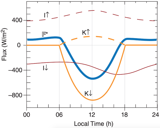
Define F* as the net radiative flux (positive upward) perpendicular to the Earth’s surface. This net flux has contributions (Figure 2.13) from downwelling solar radiation K↓ , reflected upwelling solar K↑ , downwelling longwave (IR) radiation emitted from the atmosphere I↓ , and upwelling longwave emitted from the Earth I↑:

\(\ \begin{align} \mathbb{F}^{*}=K \downarrow+K \uparrow+I \downarrow+I \uparrow\tag{2.33}\end{align}\)

where K↓ and I↓ are negative because they are downward.

Figure 2.13 Typical diurnal variation of radiative fluxes at the surface. Fluxes are positive upward.

2.4.1. Solar

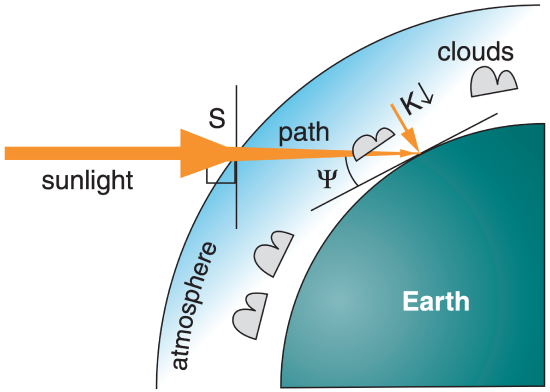
Recall that the solar irradiance (i.e., the solar constant) is S_o ≈ 1361 W·m^–2 (equivalent to 1.11 K·m s^–1 in kinematic form after dividing by ρ·C_p ) at the top of the atmosphere. Some of this radiation is attenuated between the top of the atmosphere and the surface (Figure 2.14). Also, the sine law (eq. 2.19) must be used to find the component of downwelling solar flux K↓ that is perpendicular to the surface. The result for daytime is

\(\ \begin{align}K \downarrow=-S_{o} \cdot T_{r} \cdot \sin (\Psi)\tag{2.34}\end{align}\)

where T_r is a net sky transmissivity. A negative sign is incorporated into eq. (2.34) because K↓ is a downward flux. Eq. (2.6) can be used to find sin(Ψ). At night, the downwelling solar flux is zero.

Figure 2.14 Fate of sunlight en route to the Earth’s surface

Net transmissivity depends on path length through the atmosphere, atmospheric absorption characteristics, and cloudiness. One approximation for the net transmissivity of solar radiation is

\(\ \begin{align}T_{r}=(0.6+0.2 \sin \Psi)\left(1-0.4 \sigma_{H}\right)\left(1-0.7 \sigma_{M}\right)\left(1-0.4 \sigma_{L}\right)\tag{2.35}\end{align}\)

where cloud-cover fractions for high, middle, and low clouds are σ_H, σ_M, and σ_L, respectively. These cloud fractions vary between 0 and 1, and the transmissivity also varies between 0 and 1.

Of the sunlight reaching the surface, a portion might be reflected:

\(\ \begin{align}K \uparrow=-A \cdot K \downarrow\tag{2.36}\end{align}\)

where the surface albedo is A.

Sample Application

Downwelling sunlight shines through an atmosphere with 0.8 net sky transmissivity, and hits a ground surface of albedo 0.5, at a time when sin(Ψ) = 0.3. The surface emits 400 W m^–2 IR upward into the atmosphere, and absorbs 350 W m^–2 IR coming down from the atmosphere. Find the net radiative flux.

Find the Answer

Given: Tr = 0.8, S_o = 1361 W m^–2 , A = 0.5.

I↑ = 400 W m^–2 , I↓ = 350 W m^–2

Find: F* = ? W m^–2

Use eq. (2.34):

K↓ =–(1361 W m^–2)·(0.8)· (0.3) = –327 W m^–2

Use eq. (2.36): K↑= –(0.5)·(–327 W m^–2)= 163 W m^–2

Use eq. (2.33): F* =(–327)+(163)+(–350)+(400) W m^–2

F* = –114 W m^–2

Check: Units OK. Magnitude and sign OK.

Exposition: Negative sign means net inflow to the surface, such as would cause daytime warming.

2.4.2. Longwave (IR)

Upward emission of IR radiation from the Earth’s surface can be found from the Stefan-Boltzmann relationship:

\(\ \begin{align}I \uparrow=e_{I R} \cdot \sigma_{S B} \cdot T^{4}\tag{2.37}\end{align}\)

where e_IR is the surface emissivity in the IR portion of the spectrum (e_IR = 0.9 to 0.99 for most surfaces), and σ_SB is the Stefan-Boltzmann constant (= 5.67x10^–8 W·m^–2·K^–4).

However, downward IR radiation from the atmosphere is much more difficult to calculate. As an alternative, sometimes a net longwave flux is defined by

\(\ \begin{align}I^{*}=I \downarrow+I \uparrow\tag{2.38}\end{align}\)

One approximation for this flux is

\(\ \begin{align}I^{*}=b \cdot\left(1-0.1 \sigma_{H}-0.3 \sigma_{M}-0.6 \sigma_{L}\right)\tag{2.39}\end{align}\)

where parameter b = 98.5 W·m^–2 , or b = 0.08 K·m·s^–1 in kinematic units.

2.4.3. Net Radiation

Combining eqs. (2.33), (2.34), (2.35), (2.36) and (2.39) gives the net radiation (F*, defined positive upward):

\(\ \begin{align} \mathbb{F}^{*}=-(1-A) \cdot S \cdot T_{r} \cdot \sin (\Psi)+I^{*} \quad daytime\tag{2.40a}\end{align}\)

\(\ \begin{align}=I^{*} \ \ \ \ \ \ \ \ \ \ \ nighttime \tag{2.40b}\end{align}\)

Sample Application

Find the net radiation at the surface in Vancouver, Canada, at noon (standard time) on 22 Jun. Low clouds are present with 30% coverage.

Find the Answer

Assume: Grass lawns with albedo A = 0.2 .

No other clouds.

Given: σ_L = 0.3

Find: F* = ? W·m^–2

Use ψ = 64.1° from an earlier Sample Application.​​​​​​​

Use eq. (2.35) to find the transmissivity:

T_r = [0.6+0.2·sinψ]·(1–0.4·σ_L)

= [0.6 + 0.2·sin(64.1°)]·[1–(0.4·0.3)]

= [0.80]·(0.88) = 0.686

Use eq. (2.39) to find net IR contribution:

I* = b·(1 – 0.6·σ_L)

= (98.5 W·m^–2 )·[1–(0.6·0.3)] = 80.77 W·m^–2

Use eq. (2.40a):

F* = –(1–A) · S · T_r · sin(ψ) + I*

= –(1–0.2) · (1361 W·m^–2) · 0.686 · sin(64.1°) + 80.77 W·m^–2

=( –671.89 + 80.77) W·m^–2 = –591. W·m^{–2​​​​​​​}

Check: Units OK. Physics OK.

Exposition: The surface flux is only about 43% of that at the top of the atmosphere, for this case. The negative sign indicates a net inflow of radiation to the surface, such as can cause warming during daytime.