1.4: Meteorological Concentions
- Page ID
- 9527
\( \newcommand{\vecs}[1]{\overset { \scriptstyle \rightharpoonup} {\mathbf{#1}} } \)
\( \newcommand{\vecd}[1]{\overset{-\!-\!\rightharpoonup}{\vphantom{a}\smash {#1}}} \)
\( \newcommand{\id}{\mathrm{id}}\) \( \newcommand{\Span}{\mathrm{span}}\)
( \newcommand{\kernel}{\mathrm{null}\,}\) \( \newcommand{\range}{\mathrm{range}\,}\)
\( \newcommand{\RealPart}{\mathrm{Re}}\) \( \newcommand{\ImaginaryPart}{\mathrm{Im}}\)
\( \newcommand{\Argument}{\mathrm{Arg}}\) \( \newcommand{\norm}[1]{\| #1 \|}\)
\( \newcommand{\inner}[2]{\langle #1, #2 \rangle}\)
\( \newcommand{\Span}{\mathrm{span}}\)
\( \newcommand{\id}{\mathrm{id}}\)
\( \newcommand{\Span}{\mathrm{span}}\)
\( \newcommand{\kernel}{\mathrm{null}\,}\)
\( \newcommand{\range}{\mathrm{range}\,}\)
\( \newcommand{\RealPart}{\mathrm{Re}}\)
\( \newcommand{\ImaginaryPart}{\mathrm{Im}}\)
\( \newcommand{\Argument}{\mathrm{Arg}}\)
\( \newcommand{\norm}[1]{\| #1 \|}\)
\( \newcommand{\inner}[2]{\langle #1, #2 \rangle}\)
\( \newcommand{\Span}{\mathrm{span}}\) \( \newcommand{\AA}{\unicode[.8,0]{x212B}}\)
\( \newcommand{\vectorA}[1]{\vec{#1}} % arrow\)
\( \newcommand{\vectorAt}[1]{\vec{\text{#1}}} % arrow\)
\( \newcommand{\vectorB}[1]{\overset { \scriptstyle \rightharpoonup} {\mathbf{#1}} } \)
\( \newcommand{\vectorC}[1]{\textbf{#1}} \)
\( \newcommand{\vectorD}[1]{\overrightarrow{#1}} \)
\( \newcommand{\vectorDt}[1]{\overrightarrow{\text{#1}}} \)
\( \newcommand{\vectE}[1]{\overset{-\!-\!\rightharpoonup}{\vphantom{a}\smash{\mathbf {#1}}}} \)
\( \newcommand{\vecs}[1]{\overset { \scriptstyle \rightharpoonup} {\mathbf{#1}} } \)
\( \newcommand{\vecd}[1]{\overset{-\!-\!\rightharpoonup}{\vphantom{a}\smash {#1}}} \)
\(\newcommand{\avec}{\mathbf a}\) \(\newcommand{\bvec}{\mathbf b}\) \(\newcommand{\cvec}{\mathbf c}\) \(\newcommand{\dvec}{\mathbf d}\) \(\newcommand{\dtil}{\widetilde{\mathbf d}}\) \(\newcommand{\evec}{\mathbf e}\) \(\newcommand{\fvec}{\mathbf f}\) \(\newcommand{\nvec}{\mathbf n}\) \(\newcommand{\pvec}{\mathbf p}\) \(\newcommand{\qvec}{\mathbf q}\) \(\newcommand{\svec}{\mathbf s}\) \(\newcommand{\tvec}{\mathbf t}\) \(\newcommand{\uvec}{\mathbf u}\) \(\newcommand{\vvec}{\mathbf v}\) \(\newcommand{\wvec}{\mathbf w}\) \(\newcommand{\xvec}{\mathbf x}\) \(\newcommand{\yvec}{\mathbf y}\) \(\newcommand{\zvec}{\mathbf z}\) \(\newcommand{\rvec}{\mathbf r}\) \(\newcommand{\mvec}{\mathbf m}\) \(\newcommand{\zerovec}{\mathbf 0}\) \(\newcommand{\onevec}{\mathbf 1}\) \(\newcommand{\real}{\mathbb R}\) \(\newcommand{\twovec}[2]{\left[\begin{array}{r}#1 \\ #2 \end{array}\right]}\) \(\newcommand{\ctwovec}[2]{\left[\begin{array}{c}#1 \\ #2 \end{array}\right]}\) \(\newcommand{\threevec}[3]{\left[\begin{array}{r}#1 \\ #2 \\ #3 \end{array}\right]}\) \(\newcommand{\cthreevec}[3]{\left[\begin{array}{c}#1 \\ #2 \\ #3 \end{array}\right]}\) \(\newcommand{\fourvec}[4]{\left[\begin{array}{r}#1 \\ #2 \\ #3 \\ #4 \end{array}\right]}\) \(\newcommand{\cfourvec}[4]{\left[\begin{array}{c}#1 \\ #2 \\ #3 \\ #4 \end{array}\right]}\) \(\newcommand{\fivevec}[5]{\left[\begin{array}{r}#1 \\ #2 \\ #3 \\ #4 \\ #5 \\ \end{array}\right]}\) \(\newcommand{\cfivevec}[5]{\left[\begin{array}{c}#1 \\ #2 \\ #3 \\ #4 \\ #5 \\ \end{array}\right]}\) \(\newcommand{\mattwo}[4]{\left[\begin{array}{rr}#1 \amp #2 \\ #3 \amp #4 \\ \end{array}\right]}\) \(\newcommand{\laspan}[1]{\text{Span}\{#1\}}\) \(\newcommand{\bcal}{\cal B}\) \(\newcommand{\ccal}{\cal C}\) \(\newcommand{\scal}{\cal S}\) \(\newcommand{\wcal}{\cal W}\) \(\newcommand{\ecal}{\cal E}\) \(\newcommand{\coords}[2]{\left\{#1\right\}_{#2}}\) \(\newcommand{\gray}[1]{\color{gray}{#1}}\) \(\newcommand{\lgray}[1]{\color{lightgray}{#1}}\) \(\newcommand{\rank}{\operatorname{rank}}\) \(\newcommand{\row}{\text{Row}}\) \(\newcommand{\col}{\text{Col}}\) \(\renewcommand{\row}{\text{Row}}\) \(\newcommand{\nul}{\text{Nul}}\) \(\newcommand{\var}{\text{Var}}\) \(\newcommand{\corr}{\text{corr}}\) \(\newcommand{\len}[1]{\left|#1\right|}\) \(\newcommand{\bbar}{\overline{\bvec}}\) \(\newcommand{\bhat}{\widehat{\bvec}}\) \(\newcommand{\bperp}{\bvec^\perp}\) \(\newcommand{\xhat}{\widehat{\xvec}}\) \(\newcommand{\vhat}{\widehat{\vvec}}\) \(\newcommand{\uhat}{\widehat{\uvec}}\) \(\newcommand{\what}{\widehat{\wvec}}\) \(\newcommand{\Sighat}{\widehat{\Sigma}}\) \(\newcommand{\lt}{<}\) \(\newcommand{\gt}{>}\) \(\newcommand{\amp}{&}\) \(\definecolor{fillinmathshade}{gray}{0.9}\)From René Descartes we get more than the name “Cartesian”. In 1637 he published a book Discours de la Méthode, in which he defined the principles of the modern scientific method:
- Accept something as true only if you know it to be true.
- Break difficult problems into small parts, and solve each part in order to solve the whole problem.
- Start from the simple, and work towards the com- plex. Seek relationships between the variables.
- Do not allow personal biases or judgements to interfere, and be thorough. This method formed the basis of the scientific renaissance, and marked an important break away from blind belief in philosophers such as Aristotle.
During 1970 to 2012 there were 8,835 disasters, 1.94 million deaths, and economic losses equivalent to US$ 2.4 trillion due to droughts, temperature extremes, tropical cyclones, floods, and their related health epidemics. Of these totals, storms caused 79% of the disasters, 55% of lives lost, and 86% of economic losses. Individual events included: 300,000 killed in 1970 cyclone Bhola in Bangladesh; 300,000 killed in 1983 drought in Ethiopia; 150,000 killed in drought in Sudan; and 138,866 killed in 1991 cyclone Gorky in Bangladesh. Most of the deaths were in less-developed countries, while most of the economic losses were in the most-developed countries (e.g. US$ 147 billion and $50 billion from hurricanes Katrina and Sandy in the USA). Source: WMO, 2014: “The Atlas of Mortality and Economic Losses from Weather, Climate and Water Extremes, 1970-2012”.
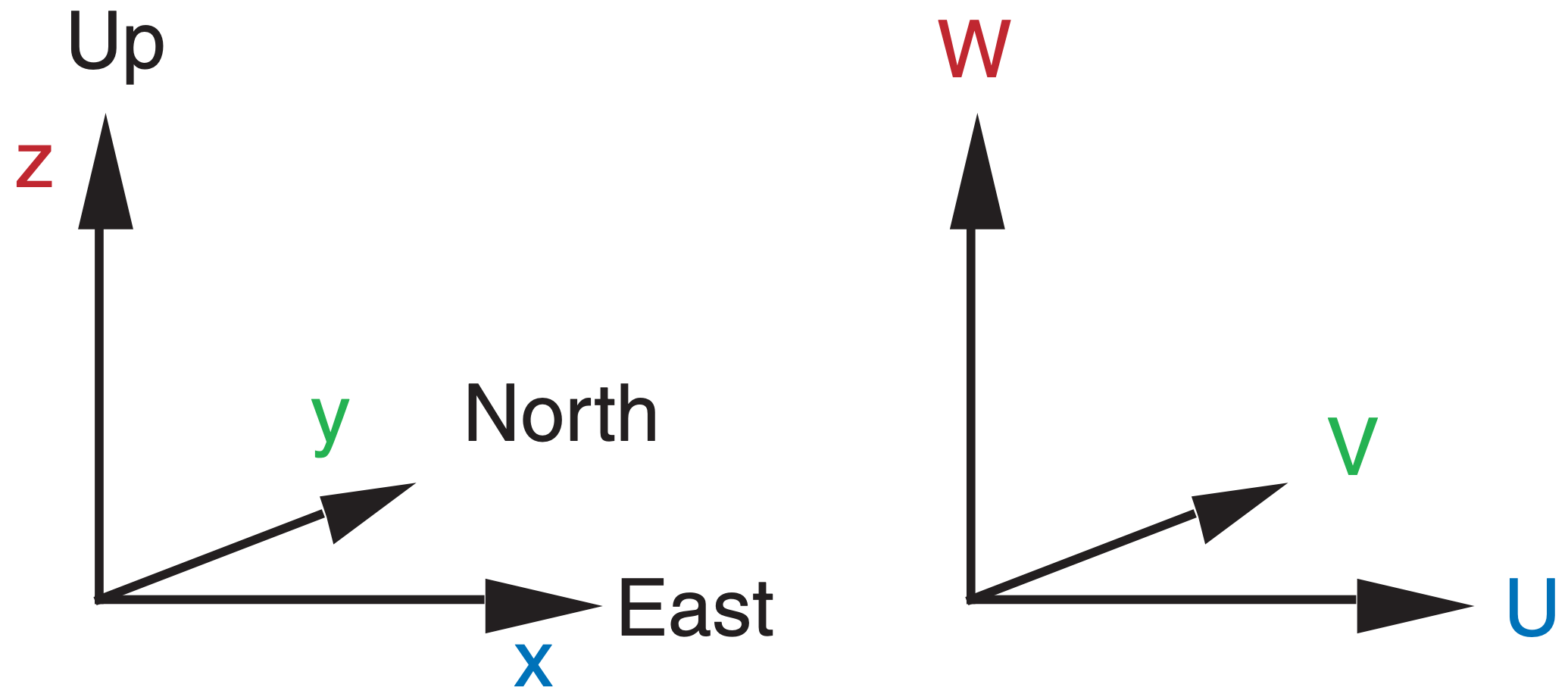
Although the Earth is approximately spherical, you need not always use spherical coordinates. For the weather at a point or in a small region such as a town, state, or province, you can use local right-hand Cartesian (rectangular) coordinates, as sketched in Figure 1.1. Usually, this coordinate system is aligned with x pointing east, y pointing north, and z pointing up. Other orientations are sometimes used. Velocity components U, V, and W correspond to motion in the x, y, and z directions. For example, a positive value of U is a velocity component from west to east, while negative is from east to west. Similarly, V is positive northward, and W is positive upward (Figure 1.1).
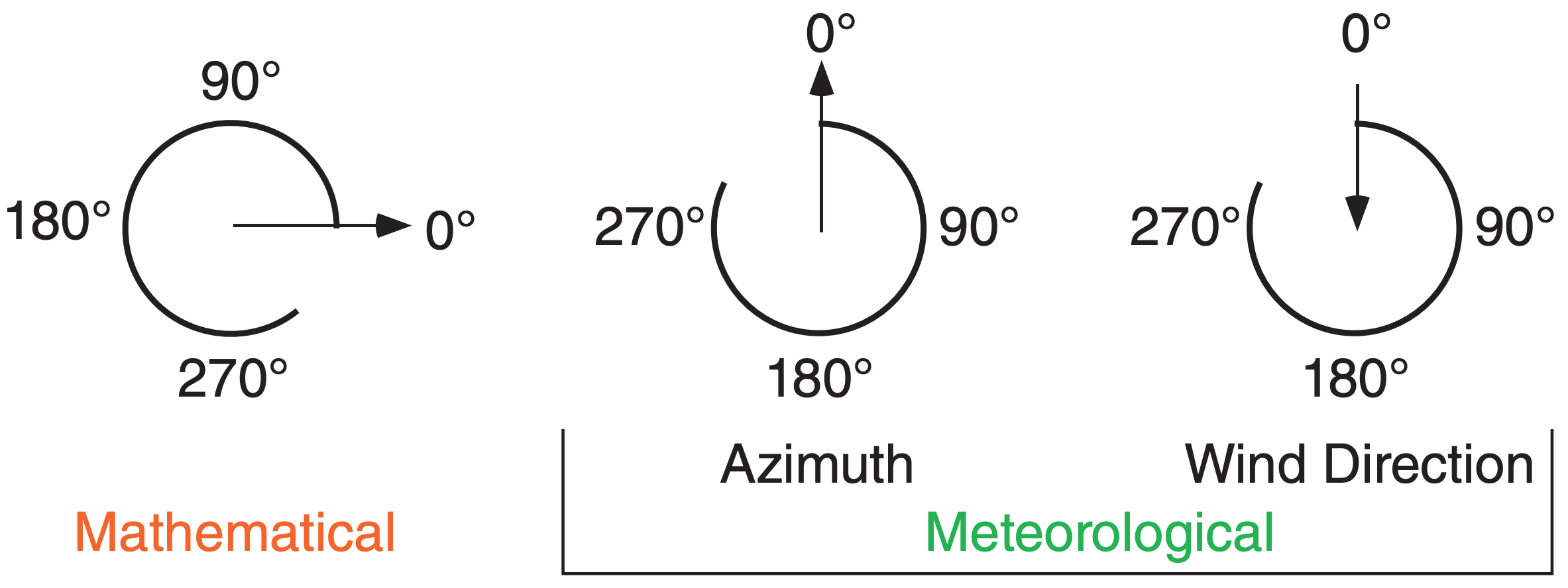
In polar coordinates, horizontal velocities can be expressed as a direction (α), and speed or magnitude (M). Historically, horizontal wind directions are based on the compass, with 0° to the north (the positive y direction), and with degrees increasing in a clockwise direction through 360°. Negative angles are not usually used. Unfortunately, this differs from the usual mathematical convention of 0° in the x direction, increasing counter-clockwise through 360° (Figure 1.2). Historically winds are named by the direction from which they come, while in mathematics angles give the direction toward which things move. Thus, a west wind is a wind from the west; namely, from 270°. It corresponds to a positive value of U, with air moving in the positive x direction. Because of these differences, the usual trigonometric equations cannot be used to convert between (U, V) and (α, M). Use the following equations instead, where α is the compass direction from which winds come.
Conversion to Speed and Direction:
\(\ \begin{align} M=\left(U^{2}+V^{2}\right)^{1 / 2} \tag{1.1} \end{align}\)
\(\ \begin{align} \alpha=90^{\circ}-\frac{360^{\circ}}{C} \cdot \arctan \left(\frac{V}{U}\right)+\alpha_{o} \tag{1.2a}\end{align}\)
where αo = 180° if U > 0, but is zero otherwise. C is the angular rotation in a full circle (C = 360° = 2·π radians).
Bullets • identify key equations that are fundamental, or are needed for understanding later chapters.
Some computer languages and spreadsheets allow a two-argument arc tangent function (atan2):
\(\ \begin{align} \alpha=\frac{360^{\circ}}{C} \cdot \operatorname{atan} 2(V, U)+180^{\circ} \tag{1.2b} \end{align}\)
In the C and C++ programming languages, you might need to switch the order of U & V
Some calculators, spreadsheets or computer functions use angles in degrees, while others use radians. If you don’t know which units are used, compute the arccos(–1) as a test. If the answer is 180, then your units are degrees; otherwise, an answer of 3.14159 indicates radians. Use whichever value of C is appropriate for your units.
Conversion to U and V:
\(\ \begin{align} U=-M\cdot sin(\alpha)\tag{1.3} \end{align}\)
\(\ \begin{align} V=-M\cdot cos(\alpha)\tag{1.4} \end{align}\)
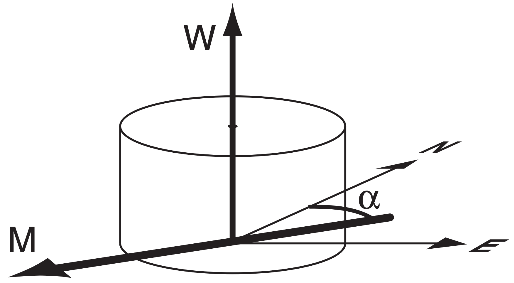
In three dimensions, cylindrical coordinates (M, α, W) are sometimes used for velocity instead of Cartesian (U, V, W), where horizontal velocity components are specified by direction and speed, and the vertical component remains W (see Figure 1.3).
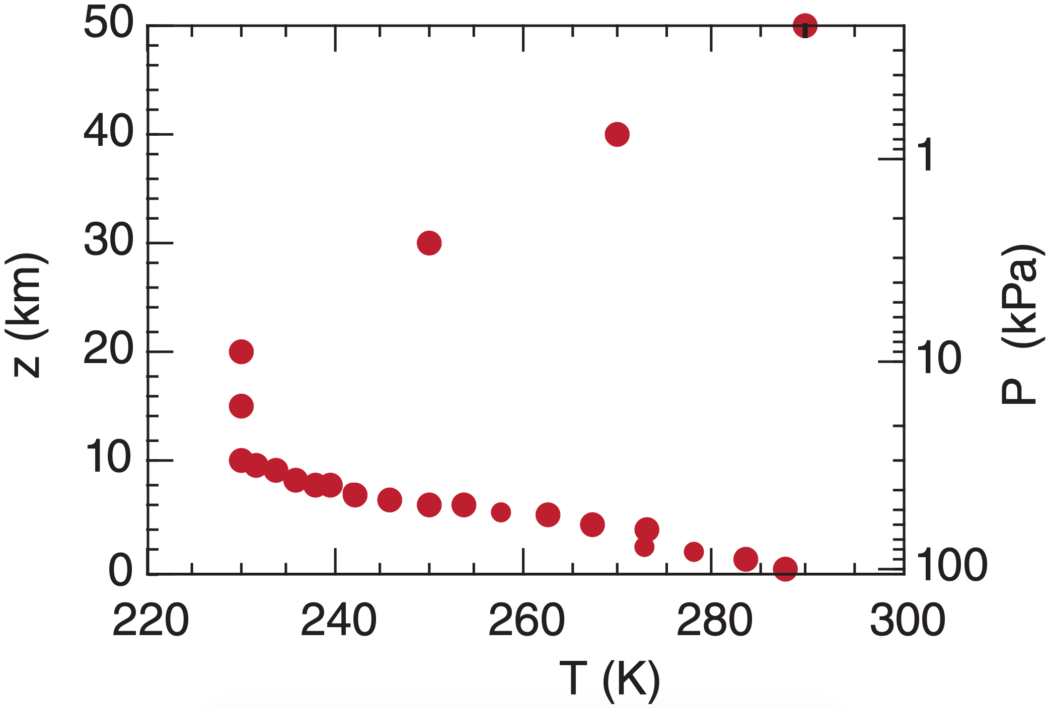
Most meteorological graphs are like graphs in other sciences, with dependent variables on the ordinate (vertical axis) plotted against an independent variable on the abscissa (horizontal axis). However, in meteorology the axes are often switched when height (z) is the independent variable. This axis switching makes locations higher in the graph correspond to locations higher in the atmosphere (Figure 1.4).
Sample Application Find wind speed and direction, given eastward component 3 m s–1, and northward 4 m s–1. Find the Answer (Problem-solving methods are given in Appendix A.) Given: U = 3 m s–1. eastward wind component. V = 4 m s–1. northward wind component. Find: M = ? m s–1. wind speed α = ? degrees. wind direction
Sketch:
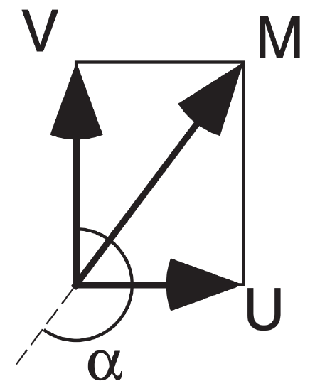
Use eq. (1.1):
M = [ U2 + V2 ] 1/2
= [ (3 m s–1)2 + (4 m s–1)2 ]0.5
= (9 + 16)0.5 \(\cdot\)[(m s–1)2]0.5
= (25)0.5 m s–1 = 5 m s–1.
Use eq. (1.2a):
α = 90° – (360°/C)·arctan(V/U) + 180°
= 90° – (360/360)·arctan[(4 m s–1)/(3 m s–1)]+180°
= 90° – tan–1(1.333) + 180°
= 90° – 53.13° + 180° = 216.87°.
Check: Units OK. Sketch OK. Values physical.
Exposition: Thus, the wind is from the south-southwest (SSW) at 5 m s–1.
