
11: A Warmer World- Temperature Effects On Chemical Reactions
- Page ID
- 34466
\( \newcommand{\vecs}[1]{\overset { \scriptstyle \rightharpoonup} {\mathbf{#1}} } \)
\( \newcommand{\vecd}[1]{\overset{-\!-\!\rightharpoonup}{\vphantom{a}\smash {#1}}} \)
\( \newcommand{\dsum}{\displaystyle\sum\limits} \)
\( \newcommand{\dint}{\displaystyle\int\limits} \)
\( \newcommand{\dlim}{\displaystyle\lim\limits} \)
\( \newcommand{\id}{\mathrm{id}}\) \( \newcommand{\Span}{\mathrm{span}}\)
( \newcommand{\kernel}{\mathrm{null}\,}\) \( \newcommand{\range}{\mathrm{range}\,}\)
\( \newcommand{\RealPart}{\mathrm{Re}}\) \( \newcommand{\ImaginaryPart}{\mathrm{Im}}\)
\( \newcommand{\Argument}{\mathrm{Arg}}\) \( \newcommand{\norm}[1]{\| #1 \|}\)
\( \newcommand{\inner}[2]{\langle #1, #2 \rangle}\)
\( \newcommand{\Span}{\mathrm{span}}\)
\( \newcommand{\id}{\mathrm{id}}\)
\( \newcommand{\Span}{\mathrm{span}}\)
\( \newcommand{\kernel}{\mathrm{null}\,}\)
\( \newcommand{\range}{\mathrm{range}\,}\)
\( \newcommand{\RealPart}{\mathrm{Re}}\)
\( \newcommand{\ImaginaryPart}{\mathrm{Im}}\)
\( \newcommand{\Argument}{\mathrm{Arg}}\)
\( \newcommand{\norm}[1]{\| #1 \|}\)
\( \newcommand{\inner}[2]{\langle #1, #2 \rangle}\)
\( \newcommand{\Span}{\mathrm{span}}\) \( \newcommand{\AA}{\unicode[.8,0]{x212B}}\)
\( \newcommand{\vectorA}[1]{\vec{#1}} % arrow\)
\( \newcommand{\vectorAt}[1]{\vec{\text{#1}}} % arrow\)
\( \newcommand{\vectorB}[1]{\overset { \scriptstyle \rightharpoonup} {\mathbf{#1}} } \)
\( \newcommand{\vectorC}[1]{\textbf{#1}} \)
\( \newcommand{\vectorD}[1]{\overrightarrow{#1}} \)
\( \newcommand{\vectorDt}[1]{\overrightarrow{\text{#1}}} \)
\( \newcommand{\vectE}[1]{\overset{-\!-\!\rightharpoonup}{\vphantom{a}\smash{\mathbf {#1}}}} \)
\( \newcommand{\vecs}[1]{\overset { \scriptstyle \rightharpoonup} {\mathbf{#1}} } \)
\(\newcommand{\longvect}{\overrightarrow}\)
\( \newcommand{\vecd}[1]{\overset{-\!-\!\rightharpoonup}{\vphantom{a}\smash {#1}}} \)
\(\newcommand{\avec}{\mathbf a}\) \(\newcommand{\bvec}{\mathbf b}\) \(\newcommand{\cvec}{\mathbf c}\) \(\newcommand{\dvec}{\mathbf d}\) \(\newcommand{\dtil}{\widetilde{\mathbf d}}\) \(\newcommand{\evec}{\mathbf e}\) \(\newcommand{\fvec}{\mathbf f}\) \(\newcommand{\nvec}{\mathbf n}\) \(\newcommand{\pvec}{\mathbf p}\) \(\newcommand{\qvec}{\mathbf q}\) \(\newcommand{\svec}{\mathbf s}\) \(\newcommand{\tvec}{\mathbf t}\) \(\newcommand{\uvec}{\mathbf u}\) \(\newcommand{\vvec}{\mathbf v}\) \(\newcommand{\wvec}{\mathbf w}\) \(\newcommand{\xvec}{\mathbf x}\) \(\newcommand{\yvec}{\mathbf y}\) \(\newcommand{\zvec}{\mathbf z}\) \(\newcommand{\rvec}{\mathbf r}\) \(\newcommand{\mvec}{\mathbf m}\) \(\newcommand{\zerovec}{\mathbf 0}\) \(\newcommand{\onevec}{\mathbf 1}\) \(\newcommand{\real}{\mathbb R}\) \(\newcommand{\twovec}[2]{\left[\begin{array}{r}#1 \\ #2 \end{array}\right]}\) \(\newcommand{\ctwovec}[2]{\left[\begin{array}{c}#1 \\ #2 \end{array}\right]}\) \(\newcommand{\threevec}[3]{\left[\begin{array}{r}#1 \\ #2 \\ #3 \end{array}\right]}\) \(\newcommand{\cthreevec}[3]{\left[\begin{array}{c}#1 \\ #2 \\ #3 \end{array}\right]}\) \(\newcommand{\fourvec}[4]{\left[\begin{array}{r}#1 \\ #2 \\ #3 \\ #4 \end{array}\right]}\) \(\newcommand{\cfourvec}[4]{\left[\begin{array}{c}#1 \\ #2 \\ #3 \\ #4 \end{array}\right]}\) \(\newcommand{\fivevec}[5]{\left[\begin{array}{r}#1 \\ #2 \\ #3 \\ #4 \\ #5 \\ \end{array}\right]}\) \(\newcommand{\cfivevec}[5]{\left[\begin{array}{c}#1 \\ #2 \\ #3 \\ #4 \\ #5 \\ \end{array}\right]}\) \(\newcommand{\mattwo}[4]{\left[\begin{array}{rr}#1 \amp #2 \\ #3 \amp #4 \\ \end{array}\right]}\) \(\newcommand{\laspan}[1]{\text{Span}\{#1\}}\) \(\newcommand{\bcal}{\cal B}\) \(\newcommand{\ccal}{\cal C}\) \(\newcommand{\scal}{\cal S}\) \(\newcommand{\wcal}{\cal W}\) \(\newcommand{\ecal}{\cal E}\) \(\newcommand{\coords}[2]{\left\{#1\right\}_{#2}}\) \(\newcommand{\gray}[1]{\color{gray}{#1}}\) \(\newcommand{\lgray}[1]{\color{lightgray}{#1}}\) \(\newcommand{\rank}{\operatorname{rank}}\) \(\newcommand{\row}{\text{Row}}\) \(\newcommand{\col}{\text{Col}}\) \(\renewcommand{\row}{\text{Row}}\) \(\newcommand{\nul}{\text{Nul}}\) \(\newcommand{\var}{\text{Var}}\) \(\newcommand{\corr}{\text{corr}}\) \(\newcommand{\len}[1]{\left|#1\right|}\) \(\newcommand{\bbar}{\overline{\bvec}}\) \(\newcommand{\bhat}{\widehat{\bvec}}\) \(\newcommand{\bperp}{\bvec^\perp}\) \(\newcommand{\xhat}{\widehat{\xvec}}\) \(\newcommand{\vhat}{\widehat{\vvec}}\) \(\newcommand{\uhat}{\widehat{\uvec}}\) \(\newcommand{\what}{\widehat{\wvec}}\) \(\newcommand{\Sighat}{\widehat{\Sigma}}\) \(\newcommand{\lt}{<}\) \(\newcommand{\gt}{>}\) \(\newcommand{\amp}{&}\) \(\definecolor{fillinmathshade}{gray}{0.9}\)Search Fundamentals of Biochemistry
Learning goals written by Claude, Anthropic)
By the end of this chapter, students should be able to:
Thermoregulation and Climate Vulnerability
- Distinguish ectothermy from endothermy and homeothermy from poikilothermy, explain why these are independent descriptors, describe the four mechanisms of heat exchange (radiation, evaporation, convection, conduction), and predict which organisms face greater direct biochemical risk from climate-driven temperature increases.
The Arrhenius Equation and Activation Energy
- State the Arrhenius equation, explain how it derives from the Maxwell-Boltzmann distribution of molecular kinetic energies, derive the two-temperature form, and use it to calculate that Ea ≈ 54 kJ/mol produces a doubling of reaction rate (Q₁₀ ≈ 2) for a 10°C increase near room temperature.
- Explain why a plot of ln k versus 1/T is linear with slope −Ea/R, interpret this relationship to extract activation energies from experimental rate data, and apply it to soil enzyme Ea values (β-glucosidase avg 44.9, cellobiohydrolase 42.0, peroxidase 33.2, phenol oxidase 58.9 kJ/mol) to predict how warming will accelerate lignocellulose decomposition and soil CO₂ release.
The Q₁₀ Temperature Coefficient
- Define Q₁₀, write and apply the equation relating Q₁₀ to rate constants and temperatures, explain why Q₁₀ is not a constant — decreasing as absolute temperature increases — and interpret Q₁₀ > 2, = 1, and < 1 in biological contexts including enzyme denaturation.
- Apply Q₁₀ reasoning to soil respiration data (annual Q₁₀ ≈ 2.76, daily average ≈ 2.04, decreasing with temperature), explain why Q₁₀ models are adequate for simple reactions but inadequate for complex anaerobic decomposition processes, and identify VCell/COPASI-style systems biology approaches as more appropriate alternatives.
Conformational Dynamics and Enzyme Catalysis
- Explain how temperature affects enzyme-catalyzed reactions through both rate constant changes and conformational flexibility, using RNase A as an example — describing how His 48, located 18 Å from the active site, regulates rate-limiting product release through coupled loop motions, and predicting the consequence of His 48 → Ala mutation on kcat.
Inspiration for the chapter comes from Biochemical Adaptation by Hochachka and Somero.
Organisms adapt to their environment, with temperature among the main drivers. This has occurred over geological time (think of arctic camels 3.4 million years ago!) and space with temperature gradients in terrestrial and aquatic environments. This is evident in the different species that thrive at different mountain heights and ocean depths. Species that can move have advantages in selecting an environment best suited to their thermal needs. Historically, homo sapiens have engaged in seasonal migration, and aquatic species in vertical migrations.
Temperature effects are universal throughout life, and physiological and biochemical adaptations are ubiquitous. Metabolically active life can exist from around -15 oC to about 121 oC (thermal saline springs). Unless greenhouse gas emissions decrease significantly from current levels, parts of the world will become increasingly uninhabitable due to high temperatures and rising sea levels. Estimates for climate refugees range from 1 billion people by 2050.
Two similar questions arise. Can organisms adapt to increasing temperatures as the climate changes, and are organisms living close to their maximal survivable temperatures?
Before we study the effects of temperature on chemical/biochemical reactions, let's review the basics of thermoregulation. The following classification of organisms by types of thermoregulation is from BioLibre text.
Types of Thermoregulation (Ectothermy vs. Endothermy)
Thermoregulation in organisms runs along a spectrum from endothermy to ectothermy. Endotherms generate most of their heat through metabolic processes and are colloquially called “warm-blooded.” Ectotherms use external sources of temperature to regulate their body temperatures. Ectotherms are colloquially called “cold-blooded” even though their body temperatures often stay within the same temperature ranges as warm-blooded animals.
Ectotherm
An ectotherm, from the Greek (ektós) “outside” and (thermós) “hot,” is an organism in which internal physiological sources of heat are of relatively small or quite negligible importance in controlling body temperature. Since ectotherms rely on environmental heat sources, they can operate at economical metabolic rates. Ectotherms usually live in environments with constant temperatures, such as the tropics or the ocean. Ectotherms have developed several behavioral thermoregulation mechanisms, such as basking in the sun to raise body temperature or seeking shade to lower it. The common frog is an ectotherm that regulates its body temperature in response to the external environment.
Endotherms
In contrast to ectotherms, endotherms regulate their body temperature through internal metabolic processes and usually maintain a narrow range of internal temperatures. Heat is usually generated by an animal’s normal metabolism, but under extreme cold or low activity, an endotherm generates additional heat by shivering. Many endotherms have more mitochondria per cell than ectotherms. These mitochondria enable them to generate heat by increasing the rate at which they metabolize fats and sugars. However, endothermic animals must sustain their higher metabolism by eating more food often. For example, a mouse (endotherm) must consume food daily to maintain its high metabolism, while a snake (ectotherm) may only eat once a month because its metabolism is much lower.
Homeothermy vs. Poikilothermy
Two other descriptors are also used. A poikilotherm is an organism whose internal temperature varies considerably. It is the opposite of a homeotherm, an organism that maintains thermal homeostasis. Poikilotherms’ internal temperature usually varies with the ambient environmental temperature, and many terrestrial ectotherms are poikilothermic. Poikilothermic animals include many species of fish, amphibians, and reptiles, as well as birds and mammals that lower their metabolism and body temperature during hibernation or torpor. Some ectotherms can also be homeotherms. For example, some tropical fish species inhabit coral reefs with such stable ambient temperatures that their internal temperatures remain constant. Figure \(\PageIndex{1}\) below shows the energy output vs temperature for a homeotherm (mouse) and a poikilotherm (lizard).
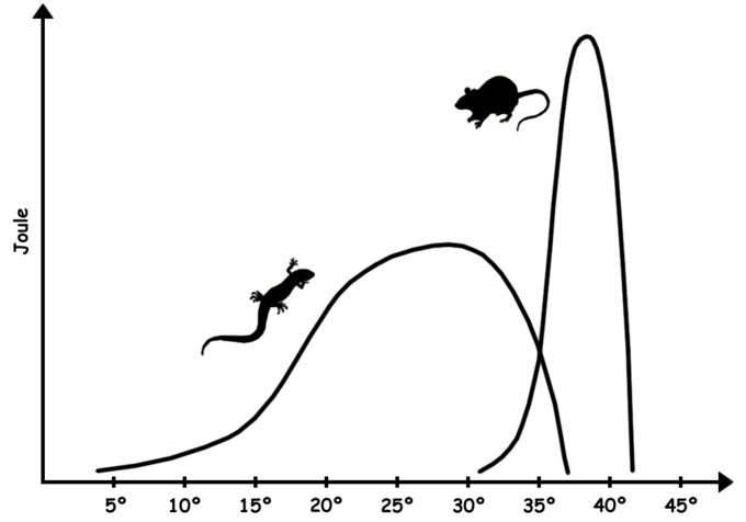 Figure \(\PageIndex{1}\): Homeotherm vs. Poikilotherm: Sustained energy output of an endothermic animal (mammal) and an ectothermic animal (reptile) as a function of core temperature. The mammal is also a homeotherm in this scenario because it maintains its internal body temperature in a very narrow range. The reptile is also a poikilotherm because it can withstand a large range of temperatures.
Another term is heterothermy, in which the temperature of a homeotherm can vary across body regions (spatially) and over time (daily or seasonally, as in hibernation). The core of a homeotherm is usually warmer than its extremities, allowing it to cool when needed. Body temperature and metabolic rate decrease during hibernation (or sustained torpor).
Means of Heat Transfer
Heat can be exchanged between an animal and its environment through four mechanisms: radiation, evaporation, convection, and conduction. Radiation is the emission of electromagnetic “heat” waves. Heat radiates from the sun and dry skin in the same manner. When a mammal sweats, evaporation removes heat from the skin's surface. Convection currents of air remove heat from the surface of dry skin as they pass over it. Heat can be conducted from one surface to another through direct contact, as when an animal rests on a warm rock.
Key Points
- Processes such as enzyme production can be modified to adapt to varying body temperatures.
- Endotherms regulate their internal body temperature independently of external temperature fluctuations, while ectotherms rely on the external environment to do so.
- Homeotherms maintain their body temperature within a narrow range, while poikilotherms can tolerate wide variations in internal body temperature, usually due to environmental conditions.
- Heat can be exchanged between the environment and animals via radiation, evaporation, convection, or conduction.
Key Terms
- ectotherm: An animal that relies on the external environment to regulate its internal body temperature.
- endotherm: An animal that regulates its internal body temperature through metabolic processes.
- homeotherm: An animal that maintains a constant internal body temperature, usually within a narrow range of temperatures.
- poikilotherm: An animal that varies its internal body temperature within a wide range of temperatures, usually as a result of variation in the environmental temperature.
These terms are diagramed below in Figure \(\PageIndex{2}\).

Figure \(\PageIndex{2}\): Thermoregulatory Term. Buffenstein et al., Biol. Rev. (2021), doi: 10.1111/brv.12791. Creative Commons Attribution License
We have discussed in the previous chapter sections how temperature can affect macromolecules such as proteins (Chapter 4) and nucleic acids (Chapter 9.1), as well as supramolecular assemblies such as membranes (Chapter 10.3). Temperature effects on small molecules and ions (such as salts in the Hofmeister series and glycerol, Chapter 4.9) in the environment that regulate the function/activity of these larger molecules and assemblies are also important. Hence, we'll review and discuss the effects of temperature on these key molecular species in the next chapter section. First, we'll delve deeper into the general impact of temperature on chemical and biochemical reactions.
Temperature Effects on the Rates of Chemical Reactions
To understand how temperature affects metabolic processes, let's first review its effects on ordinary chemical and biochemical reactions. You may remember the general rule that the rate of a chemical reaction approximately doubles when the temperature increases by 10 °C (10 K). How does that arise? This is generally true in a specific temperature range, as shown below.
The rates of reactions, either endothermic or exothermic, depend on the activation energy (Ea). The activation energy is required to move from a reactant to the transition state, which can then form the product.
The activation energy can be obtained from the Arrhenius equation (that you learned in introductory chemistry), which shows how the rate of an individual chemical reaction depends on temperature.
\begin{equation}
k=A e^{-E_a / R T}
\end{equation}
where k is the rate constant, Ea is the activation energy, Ea/RT is the average kinetic energy, and A is a constant (the "preexponential" factor).
By taking the natural log (ln) of each side and rearranging the equation, you get a "linearized" equation that is easier for most.
\begin{equation}
\ln k=\ln A-\frac{E_a}{R T}
\end{equation}
A plot of ln k vs 1/T has a slope = Ea/R, from which the activation energy can be calculated.
An alternative form can be derived:
\begin{equation}
\ln \frac{k_2}{k_1}=\frac{E_a}{R}\left(\frac{1}{T_1}-\frac{1}{T_2}\right)
\end{equation}
Here it is!
- Derivation
-
From
\begin{equation}
\ln k_1=\ln (A)-E_a / R T_1
\end{equation}Solve for lnA
\begin{equation}
\ln (A)=\ln \left(k_1\right)+E_a / R T_1
\end{equation}Substituting into the equation for ln(k2) gives
\begin{equation}
\ln \left(k_2\right)=\ln \left(k_1\right)+E_a / R T_1-E_a / R T_2
\end{equation}Rearrange to get
\begin{equation}
\ln \left(k_2\right)-\ln \left(k_1\right)=E_a / R T_1-E_a / R T_2
\end{equation}Simplify to get the final equation!
\begin{equation}
\ln \left(\frac{k_2}{k_1}\right)=\frac{E_a}{R}\left(\frac{1}{T_1}-\frac{1}{T_2}\right)
\end{equation}
Solving for Ea gives
\begin{equation}
E_a=\frac{R \ln \frac{k_2}{k_1}}{\frac{1}{T_1}-\frac{1}{T_2}}
\end{equation}
Let's use this equation to calculate an Ea that will give a doubling of the reaction rate (k2/k1 = 2) going from T1 = 295 K (21.9 0C, 71.3 o F) to T2 = 305 K (21.9 0C, 89.3 oF), a 10 oC temperature rise.
\begin{equation}
\begin{aligned}
E_a & =\frac{(8.314)(\ln 2)}{\frac{1}{295}-\frac{1}{305}} \\
& =\frac{\left(8.314 \mathrm{~J} \mathrm{~mol}^{-1} \mathrm{~K}^{-1}\right)(0.693)}{0.00339 \mathrm{~K}^{-1}-0.00328 \mathrm{~K}^{-1}} \\
& =\frac{5.76 \mathrm{Jmol}^{-1} \mathrm{~K}^{-1}}{\left(0.00011 \mathrm{~K}^{-1}\right)} \\
& =52,400 \mathrm{Jmol}^{-1}=52.4 \mathrm{~kJ} \mathrm{~mol}^{-1}
\end{aligned}
\end{equation}
Hence, if a reaction has an activation energy Ea of about 54 kJ/mol, increasing the temperature from 295 to 305 0C, (i.e., by 10 0C), doubles the reaction rate.
Assuming the activation energy is constant, the rate constants increase with temperature because a larger fraction of molecules has the energy (> Ea) required to react. This is illustrated in Figure \(\PageIndex{3}\) below.

Figure \(\PageIndex{3}\): Plot of a Maxwell-Boltzmann distribution of speeds for different temperatures T=100K, T=1200K, T=5000K. Points along the curve show (1) most likely speed, (2) average speed, and (3) thermal speed (velocity that a particle in a system would have if its kinetic energy were equal to the average energy of all the particles of the system). https://commons.wikimedia.org/wiki/F...xis-labels.svg. Creative Commons Attribution-Share Alike 4.0 International license.
Let's look at the brown vertical line around 950 m/s. If we take that as the activation energy, very few molecules in the blue distribution have the required kinetic energy > Eact to overcome it. At progressively higher temperatures, great fractions (as measured by the area under the curve to the right of the dotted line at 950 m/s) have the required energy; hence, the rates increase with temperature.
When the temperature change is 10oC, the ratio of the rate constants (or rates), k2/k1 is often called Q10, the temperature coefficient (unitless). Q10 is not a constant since it depends on the two temperatures that differ by 10 0C (10 K). Hence, the Q10 value for the 100 range from 273-283K differs from the Q10 value from 373-383K). For many reactions, Q10 is around 2 (doubling the reaction rate) - 3 (tripling the reaction rate) at physiological temperature. Q10 =2 for a given Ea only at one set of temperatures that differ by 10 oC. The variation in Q10 values is illustrated in Table \(\PageIndex{1}\) below for a reaction in which Ea = 44.5 kJ/mol. Q10 decreases from 2 as the temperatures T1 and T2 = T1+10 oC increase.
| T1 in K (oC) | T2 (K) (oC) | k2/k1 (Q10) |
| 273 (- 0.15 oC) | 283 (9.85 oC)oC | 2 |
| 373 (99.9 oC) | 383 (110 oC) | 1.45 |
| 473 (200 oC) | 483 (210 oC) | 1.26 |
Table \(\PageIndex{1}\): Q10 = k2/k1 values at different temperatures T1 and T2 that differ by 10o C.
We will see how this is important in biological settings in a bit. If Q10 = 1, the reaction is independent of temperature, and a Q10 <1 indicates a reaction that is not functioning. An example might be an enzyme-catalyzed reaction in which the threshold is reached at a higher temperature, T2 = T1 + 10, at which the enzymes lose an active conformation and start to unfold.
The same equation and the Q10parameters apply to enzyme-catalyzed reactions. The activation energies (Ea) for four enzymes involved in the degradation of lignocellulose in the surface soil and subsoil are shown in Table \(\PageIndex{2}\) below. The enzymes include two hydrolases, β-glucosidase (BG) and cellobiohydrolase (CB), which cleave cellulose, and two oxidases, peroxidase (PER) and phenol oxidase (POX), which help degrade lignin. The average Ea for these enzymes is about 44.7 kJ/mol, similar to the example in Table 1 above.
| Soil | Type | Ea (kJ/mol) | |||
| BG | CB | PER | POX | ||
| Arctic | surface | 35.4 | 39.4 | 12.7 | 81.8 |
| Subarctic | surface | 36.5 | 38.6 | 21.1 | 45.7 |
| subsoil | 52.2 | 41.5 | 22.4 | 39.4 | |
| Temperate 1 | surface | 40.9 | 38 | 64.9 | 102 |
| subsoil | 49.4 | 21.2 | 28 | 94.8 | |
| Temperate 2 | surface | 31 | 43.4 | 25.4 | 49.5 |
| subsoil | 40.9 | 39.9 | 19.8 | 47.5 | |
| Temperate 3 | surface | 51.5 | 53.6 | 28.8 | 73.2 |
| subsoil | 58.8 | 46.7 | 54.2 | 29 | |
| Tropical 1 | surface | 47.8 | 50.5 | 26.5 | 47.7 |
| subsoil | 56.6 | 47 | 47.1 | 27.1 | |
| Tropical 2 | surface | 39.3 | 42.5 | 58.3 | 82.5 |
| subsoil | 42.8 | 43.3 | 22.8 | 45.5 | |
| Avg | 44.9 | 42.0 | 33.2 | 58.9 | |
Table \(\PageIndex{2}\): Activation Energies (Ea, kJ mol−1) for extracellular soil enzymes involved in the degradation of lignocellulose.Adapted from Steinweg JM et al. (2013) PLOS ONE 8(3): e59943. https://doi.org/10.1371/journal.pone.0059943. Creative Commons CC0 public domain
Q10temperature coefficients are also used to describe biological processes such as respiration, neural signal propagation, and metabolic rates. Many biological processes are affected by temperature, especially in ectotherms, which adjust their body temperatures to their environments, including daily and seasonal temperature shifts. Mammals and birds alter their metabolic rates with temperature, as do hibernating animals.
The Q10 temperature coefficient is the factor by which the reaction rates (k or R) increase (factor of 2, 3, 1.5, etc) for each 10-degree K or C temperature increase. The following equation gives it:
\begin{equation}
Q_{10}=\left(\frac{k_2}{k_1}\right)^{10^{\circ} \mathrm{C} /\left(T_2-T_1\right)}
\end{equation}
It is also called the van't Hoff's temperature coefficient. To help understand Q10, let's consider some examples.
- If T2 - T1 = 10o, Q10 = k2/k1 for the specified temperature pairs separated by a 100 C range (T1 and T2=T1+10). Remember that Q10 is not a constant; it depends on the temperature pairs and decreases with increasing temperature.
- If the temperature range is > 100 C, the the measured ratio k2/k1 is a factor > 1 x Q10
- If the temperature range is < 100 C, the the measured ratio k2/k1 is a fraction of Q10
This equation can be converted to
\begin{equation}
k_2=k_1 Q_{10}^{\left(T_2-T_1\right) / 10^{\circ} \mathrm{C}}
\end{equation}
where the rate constant k2 is related to a "base" rate k1 at a base temperature of T1. Figure \(\PageIndex{4}\) below shows an interactive graph of the above equation.
Figure \(\PageIndex{4}\): Interactive graph of k2 (rate 2) vs. delta T at different base rates k1.
Change the base rate constant, k1, at a base temperature of T1 and Q10 coefficient to see how they affect k2.
Note that if Q10 =1, then k2 at T1 + 10 = k1 at T1, so the rate is independent of the temperature.
For most biological systems, the Q10 value is ~ 2 to 3 under physiologically relevant conditions. The ratios of the rates (R2/R1) for different Q10 values are shown in Figure \(\PageIndex{5}\) below.

Figure \(\PageIndex{5}\): Idealized graphs showing the dependence on temperature of the rates of chemical reactions and various biological processes for several different Q10 temperature coefficients. The dots on the graph show how the rate changes with a 10 °C change in temperature. Wikipedia. https://en.wikipedia.org/wiki/Q10_(t...e_coefficient). CC BY-SA 4.0
Again, this hypothetical graph shows the general meaning of Q10 values.
The "Q" model has been used to fit complex reaction systems, not just individual reactions. Figure \(\PageIndex{6}\) below shows the daily mean soil respiration rate as a function of soil temperature. In these graphs, the x-axis is Temperature, not ΔT.

Figure \(\PageIndex{6}\): Relationships between daily mean soil respiration (Rs) and soil temperature (Ts). Jia X et al., PLoS ONE 8(2): e57858. https://doi.org/10.1371/journal.pone.0057858. Creative Commons Attribution License
The soil temperature, Ts, was measured at a depth of 10 cm. Open circles are from January to June; closed circles are from July to December. The solid lines use a Q10 model, in which the observed Rs vs. Ts data are fit with an equation that optimizes the Q10 parameter. The dashed lines are fitted using a logistic model we used in Chapter 5.7 to fit ELISA data. Rs is significantly different between the first and second halves of the year.
The soil respiration rate, Rs, at 10 cm depth was strongly affected by temperature, with an annual Q10 value of 2.76. Daily estimates of Q10 averaged 2.04 and decreased with increasing Ts. A study of seagrass showed that Q10 values are affected by plant tissue age and that Q10 varies significantly with initial temperature and temperature range.
The use of Q10 values from the Arrhenius equation assumes that chemical and biochemical processes are exponential functions of temperature. For complex processes such as the decomposition of organic matter, it is better to model the entire system by accounting for the individual enzymes involved. One problem with using Q10 values for very complex systems is the choice of the base temperature value for rate comparisons. The anaerobic decomposition of organic matter is generally a linear function of temperature between 5°C and 30°C, suggesting that a Q10-based model is not ideal. A more complex systems biology approach using programs such as Vcell and COPASI would be preferable and less likely to lead to errors in predicted CH4 emissions from decomposition.
Getting Back to Proteins
Chapter 6.1 explored the mechanisms enzymes use to catalyze chemical reactions. These included general acid/base catalysis, metal ion (electrostatic) catalysis, covalent (nucleophilic) catalysis, and transition state stabilization. Some physical processes included intramolecular catalysis and strain/distortion. The rate-limiting step in enzyme-catalyzed reactions can involve bond breaking in the substrate, product dissociation, and conformational changes required to facilitate binding, catalysis, and dissociation. A rate-limiting conformational change may occur not in the active-site pocket but in nearby loops that modulate the accessibility of the reactant to and the dissociation of the product from the active site. These all may be influenced by temperature, with localized conformational flexibility especially important.
An interesting example of localized conformational changes affecting enzyme activity is RNase A. His 48, 18 Å from the enzyme active site, is involved in the rate-limiting step involving product release.
Figure \(\PageIndex{7}\) shows an interactive iCn3D modelof bovine pancreatic Ribonuclease A in complex with 3'-phosphothymidine (3'-5')-pyrophosphate adenosine 3'-phosphate (1U1B)
.png?revision=1)
 Figure \(\PageIndex{7}\): Bovine pancreatic Ribonuclease A in complex with 3'-phosphothymidine (3'-5')-pyrophosphate adenosine 3'-phosphate (1U1B). (Copyright; author via source). Click the image for a popup or use this external link: https://structure.ncbi.nlm.nih.gov/i...SnrGYXSVXcLCk6
The substrate is shown in spacefill. The active site side chains and distal His 48 are shown as sticks and labeled. Two flexible loops, Loop 1 (magenta) near His 48 and Loop 4 (cyan) near the active site, are highlighted. During ligand binding, the loops move by a few angstroms, closing the active site and inhibiting product release. Product release is associated with mobile regions, including Loops 1 (20 Å from the active site) and 2. Loop 4, near the active site, is involved in the specificity for purines 5' to the substrate cleavage site. His 48 is conserved in pancreatic RNase A. If mutated to alanine, the kcat decreases by more than 10X, indicating a change in the rate-determining conformational motion. The enzyme is still very active compared to the uncatalyzed reaction. His 48 appears to regulate the rate-limiting coupled motions in the protein.
Figure \(\PageIndex{8}\) below shows the subtle shift in the conformation of apo-RNase A (magenta, no ligand, 1FS3) to the substrate-bound form (cyan, ligand in sticks, 1U1B). Note the small motion in His 48, shown in the sticks at the bottom of the animated image.
Figure \(\PageIndex{8}\): Conformational changes apo-RNase A (magenta, no ligand, 1FS3) on conversion to the substrate-bound form (cyan, ligand in sticks, 1U1B).
We will explore the effects of temperature on protein structure and function further in the next chapter section.
Summary
(Summary written by Claude, Anthropic)
This chapter establishes the physical chemistry and biological context for understanding how temperature — and therefore climate change — affects the rates of chemical and biochemical reactions, providing the quantitative foundation for the two subsequent sections on protein adaptation and ecological consequences.
Thermoregulation and climate vulnerability. Organisms regulate body temperature along a spectrum from endothermy (internal metabolic heat generation, as in mammals and birds) to ectothermy (dependence on external heat sources, as in fish, amphibians, and reptiles). Endotherms maintain narrow internal temperature ranges and require frequent feeding to sustain high metabolic rates; ectotherms operate more economically but track environmental temperatures closely. These strategies are further characterized as homeothermy (narrow internal temperature range) versus poikilothermy (wide tolerance). Critically, ectothermic poikilotherms — including most marine invertebrates, fish, and insects — have internal temperatures that directly follow environmental conditions, making their biochemistry immediately sensitive to climate warming. Two overarching questions motivate the rest of this chapter section: Can organisms adapt to rising temperatures fast enough, and are many species already operating close to their thermal limits?
The Arrhenius equation and activation energy. The rate constant of any chemical reaction depends exponentially on temperature according to the Arrhenius equation: k = Ae−Ea/RT. The physical basis is the Maxwell-Boltzmann distribution of molecular kinetic energies: at higher temperatures, a larger fraction of molecules possesses kinetic energy exceeding the activation energy threshold Ea, producing exponentially more frequent productive collisions. A linearized form (ln k = ln A − Ea/RT) allows activation energies to be extracted from the slope of ln k versus 1/T plots. A two-temperature form of the equation permits direct calculation of how a rate constant changes between any two temperatures given Ea. For a reaction with Ea ≈ 54 kJ/mol, a 10°C temperature increase near room temperature doubles the rate constant — the origin of the familiar "doubling rule."
The Q₁₀ temperature coefficient. When the temperature interval is exactly 10°C, the ratio k₂/k₁ is defined as Q₁₀, the temperature coefficient. For most biochemical reactions at physiological temperatures, Q₁₀ falls between 2 and 3. A Q₁₀ of 1 indicates complete temperature independence; a Q₁₀ below 1 signals a process being impaired at the higher temperature — for example, an enzyme losing its active conformation. Crucially, Q₁₀ is not a constant: it decreases as absolute temperature increases (demonstrated numerically for Ea = 44.5 kJ/mol across 273–483 K). This means the temperature sensitivity of biochemical processes is greatest at low baseline temperatures — directly relevant to the vulnerability of cold-adapted and polar species to modest warming. Q₁₀ reasoning extends beyond individual reactions to complex biological processes including soil respiration (measured annual Q₁₀ ≈ 2.76 in one study, with daily averages of 2.04 declining with increasing temperature), seagrass metabolism, and whole-organism metabolic rates. Activation energies for real extracellular soil enzymes — β-glucosidase (avg Ea 44.9 kJ/mol), cellobiohydrolase (42.0 kJ/mol), peroxidase (33.2 kJ/mol), and phenol oxidase (58.9 kJ/mol) — are consistent with Q₁₀ ≈ 2, confirming that warming will accelerate lignocellulose decomposition and soil CO₂ release in a positive climate feedback. However, for highly complex processes such as anaerobic decomposition (which is linear in temperature from 5–30°C), Q₁₀ models are inadequate, and mechanistic systems biology approaches are preferable.
Temperature, conformational dynamics, and enzyme function. Temperature affects enzyme-catalyzed reactions not only by changing rate constants but also by altering protein conformational flexibility, which modulates the rate-limiting step. RNase A provides a detailed example: His 48, located 18 Å from the active site, is involved in the rate-limiting product release step through coupled conformational motions in Loops 1 and 2. Mutation of His 48 to alanine reduces kcat by more than 10-fold, confirming that distal residues regulating protein dynamics can be as important for catalysis as active-site residues. Loop 4, near the active site, controls substrate specificity. These localized dynamic processes are temperature-sensitive, connecting molecular flexibility directly to the temperature dependence of enzyme activity — a theme developed fully in the following chapter section on thermal adaptation of proteins.