
5: Biofuels A - Corn and Sugar Cane Ethanol
- Page ID
- 34460
\( \newcommand{\vecs}[1]{\overset { \scriptstyle \rightharpoonup} {\mathbf{#1}} } \)
\( \newcommand{\vecd}[1]{\overset{-\!-\!\rightharpoonup}{\vphantom{a}\smash {#1}}} \)
\( \newcommand{\dsum}{\displaystyle\sum\limits} \)
\( \newcommand{\dint}{\displaystyle\int\limits} \)
\( \newcommand{\dlim}{\displaystyle\lim\limits} \)
\( \newcommand{\id}{\mathrm{id}}\) \( \newcommand{\Span}{\mathrm{span}}\)
( \newcommand{\kernel}{\mathrm{null}\,}\) \( \newcommand{\range}{\mathrm{range}\,}\)
\( \newcommand{\RealPart}{\mathrm{Re}}\) \( \newcommand{\ImaginaryPart}{\mathrm{Im}}\)
\( \newcommand{\Argument}{\mathrm{Arg}}\) \( \newcommand{\norm}[1]{\| #1 \|}\)
\( \newcommand{\inner}[2]{\langle #1, #2 \rangle}\)
\( \newcommand{\Span}{\mathrm{span}}\)
\( \newcommand{\id}{\mathrm{id}}\)
\( \newcommand{\Span}{\mathrm{span}}\)
\( \newcommand{\kernel}{\mathrm{null}\,}\)
\( \newcommand{\range}{\mathrm{range}\,}\)
\( \newcommand{\RealPart}{\mathrm{Re}}\)
\( \newcommand{\ImaginaryPart}{\mathrm{Im}}\)
\( \newcommand{\Argument}{\mathrm{Arg}}\)
\( \newcommand{\norm}[1]{\| #1 \|}\)
\( \newcommand{\inner}[2]{\langle #1, #2 \rangle}\)
\( \newcommand{\Span}{\mathrm{span}}\) \( \newcommand{\AA}{\unicode[.8,0]{x212B}}\)
\( \newcommand{\vectorA}[1]{\vec{#1}} % arrow\)
\( \newcommand{\vectorAt}[1]{\vec{\text{#1}}} % arrow\)
\( \newcommand{\vectorB}[1]{\overset { \scriptstyle \rightharpoonup} {\mathbf{#1}} } \)
\( \newcommand{\vectorC}[1]{\textbf{#1}} \)
\( \newcommand{\vectorD}[1]{\overrightarrow{#1}} \)
\( \newcommand{\vectorDt}[1]{\overrightarrow{\text{#1}}} \)
\( \newcommand{\vectE}[1]{\overset{-\!-\!\rightharpoonup}{\vphantom{a}\smash{\mathbf {#1}}}} \)
\( \newcommand{\vecs}[1]{\overset { \scriptstyle \rightharpoonup} {\mathbf{#1}} } \)
\(\newcommand{\longvect}{\overrightarrow}\)
\( \newcommand{\vecd}[1]{\overset{-\!-\!\rightharpoonup}{\vphantom{a}\smash {#1}}} \)
\(\newcommand{\avec}{\mathbf a}\) \(\newcommand{\bvec}{\mathbf b}\) \(\newcommand{\cvec}{\mathbf c}\) \(\newcommand{\dvec}{\mathbf d}\) \(\newcommand{\dtil}{\widetilde{\mathbf d}}\) \(\newcommand{\evec}{\mathbf e}\) \(\newcommand{\fvec}{\mathbf f}\) \(\newcommand{\nvec}{\mathbf n}\) \(\newcommand{\pvec}{\mathbf p}\) \(\newcommand{\qvec}{\mathbf q}\) \(\newcommand{\svec}{\mathbf s}\) \(\newcommand{\tvec}{\mathbf t}\) \(\newcommand{\uvec}{\mathbf u}\) \(\newcommand{\vvec}{\mathbf v}\) \(\newcommand{\wvec}{\mathbf w}\) \(\newcommand{\xvec}{\mathbf x}\) \(\newcommand{\yvec}{\mathbf y}\) \(\newcommand{\zvec}{\mathbf z}\) \(\newcommand{\rvec}{\mathbf r}\) \(\newcommand{\mvec}{\mathbf m}\) \(\newcommand{\zerovec}{\mathbf 0}\) \(\newcommand{\onevec}{\mathbf 1}\) \(\newcommand{\real}{\mathbb R}\) \(\newcommand{\twovec}[2]{\left[\begin{array}{r}#1 \\ #2 \end{array}\right]}\) \(\newcommand{\ctwovec}[2]{\left[\begin{array}{c}#1 \\ #2 \end{array}\right]}\) \(\newcommand{\threevec}[3]{\left[\begin{array}{r}#1 \\ #2 \\ #3 \end{array}\right]}\) \(\newcommand{\cthreevec}[3]{\left[\begin{array}{c}#1 \\ #2 \\ #3 \end{array}\right]}\) \(\newcommand{\fourvec}[4]{\left[\begin{array}{r}#1 \\ #2 \\ #3 \\ #4 \end{array}\right]}\) \(\newcommand{\cfourvec}[4]{\left[\begin{array}{c}#1 \\ #2 \\ #3 \\ #4 \end{array}\right]}\) \(\newcommand{\fivevec}[5]{\left[\begin{array}{r}#1 \\ #2 \\ #3 \\ #4 \\ #5 \\ \end{array}\right]}\) \(\newcommand{\cfivevec}[5]{\left[\begin{array}{c}#1 \\ #2 \\ #3 \\ #4 \\ #5 \\ \end{array}\right]}\) \(\newcommand{\mattwo}[4]{\left[\begin{array}{rr}#1 \amp #2 \\ #3 \amp #4 \\ \end{array}\right]}\) \(\newcommand{\laspan}[1]{\text{Span}\{#1\}}\) \(\newcommand{\bcal}{\cal B}\) \(\newcommand{\ccal}{\cal C}\) \(\newcommand{\scal}{\cal S}\) \(\newcommand{\wcal}{\cal W}\) \(\newcommand{\ecal}{\cal E}\) \(\newcommand{\coords}[2]{\left\{#1\right\}_{#2}}\) \(\newcommand{\gray}[1]{\color{gray}{#1}}\) \(\newcommand{\lgray}[1]{\color{lightgray}{#1}}\) \(\newcommand{\rank}{\operatorname{rank}}\) \(\newcommand{\row}{\text{Row}}\) \(\newcommand{\col}{\text{Col}}\) \(\renewcommand{\row}{\text{Row}}\) \(\newcommand{\nul}{\text{Nul}}\) \(\newcommand{\var}{\text{Var}}\) \(\newcommand{\corr}{\text{corr}}\) \(\newcommand{\len}[1]{\left|#1\right|}\) \(\newcommand{\bbar}{\overline{\bvec}}\) \(\newcommand{\bhat}{\widehat{\bvec}}\) \(\newcommand{\bperp}{\bvec^\perp}\) \(\newcommand{\xhat}{\widehat{\xvec}}\) \(\newcommand{\vhat}{\widehat{\vvec}}\) \(\newcommand{\uhat}{\widehat{\uvec}}\) \(\newcommand{\what}{\widehat{\wvec}}\) \(\newcommand{\Sighat}{\widehat{\Sigma}}\) \(\newcommand{\lt}{<}\) \(\newcommand{\gt}{>}\) \(\newcommand{\amp}{&}\) \(\definecolor{fillinmathshade}{gray}{0.9}\)(Learning goals written by Claude, Anthropic)
By the end of this chapter, students should be able to:
Ethanol Production: Feedstocks and Fermentation
- Compare the energy densities of ethanol, octane, hydrogen, and biodiesel using standard combustion enthalpies (kJ/g), explain why bioethanol releases ~63% of the energy of gasoline per gram, and write the three coupled equations that describe why bioethanol is theoretically carbon-neutral while identifying what those equations omit.
- Describe the four generations of bioethanol feedstocks, explain the key enzymatic steps converting corn starch to glucose — including α-amylase (endoglucosidase, retention of configuration), β-amylase (exoglucosidase, inversion of configuration), and glucoamylase (cleaves both α(1,4) and α(1,6) bonds) — and connect the retention vs. inversion mechanisms to SN2-like versus double-displacement mechanisms at the anomeric carbon.
- Describe the structure of the invertase (SInv) homooctamer from S. cerevisiae — explaining how identical subunits form two types of dimers (closed AB/CD with hydrophobic active-site floor; open EF/GH with an additional Asp-Lys salt bridge) — and explain the double-displacement retention mechanism by which Asp22 forms a glycosyl-enzyme intermediate and Glu203 acts as general acid/base to hydrolyze sucrose to glucose and fructose.
Life Cycle Analysis: Is Bioethanol Better Than Fossil Fuels?
- Define life cycle analysis (LCA), carbon intensity (CO₂ equiv per unit of activity), and global warming potential (GWP₁₀₀), write the GWP₁₀₀ equation incorporating CH₄ (GWP ≈ 28) and N₂O (GWP ≈ 265), and explain why N₂O emissions from nitrogen fertilizers are a major hidden cost of bioethanol production.
- Interpret the Lark et al. corn ethanol LCA — including how the Renewable Fuel Standards increased corn cultivation by 2.8 Mha, fertilizer use by 3–8%, and N₂O emissions, producing a carbon intensity ≥24% higher than gasoline — and explain why studies that ignore land-use change emissions systematically underestimate corn ethanol's true carbon intensity.
- Use dimensional analysis to convert the sugar cane LCA result from kg CO₂ equiv per ton of sugar cane at the farm gate (53.6 kg/ton) to kg CO₂ equiv per liter of ethanol, add the plant-gate contribution (0.60 kg/L), and apply an energy-content correction factor (33.6/21.2 MJ) to compare sugar cane bioethanol (~0.95 kg CO₂ equiv per gasoline-equivalent liter) to gasoline (~2.3 kg CO₂ equiv/L).
Biofuels vs. Solar: The Opportunity Cost Argument
- Quantify the land-use opportunity cost of biofuels by comparing the energy yield per hectare of corn bioethanol (~22,000 km of EV driving) to solar panels (~3 million km), explain why 1.5 million hectares of solar would meet all US driving needs versus the 25 million hectares of corn now used for bioethanol covering only 10% of driving fuel, and articulate why this comparison represents a fundamental policy choice rather than merely a technical one.
- Identify at least three additional negative environmental impacts of sugarcane bioethanol beyond climate change — including freshwater and marine eutrophication, particulate matter formation, and terrestrial acidification — and explain why a complete LCA must account for all of these, not only CO₂ equivalent emissions.
Introduction
The world has a great need for energy. We have invested vast sums of money in finding and using fossil fuels. At first glance, fossil fuels appear to be an ideal energy source since they are highly reduced, easily stored, energy-dense, and abundant. Yet we now know the immense cost of their use: pollution that shortens lives and climate change. We have dramatically increased our bioethanol production from corn and sugar cane to reduce our reliance on fossil fuels for transportation. Ethanol is partially oxidized as it has one oxygen atom in the two-carbon molecule. Hence, the energy released per gram is about 63% (by mass) and 70% (by volume) of that of gasoline. The energy values for various fuels are shown in Table \(\PageIndex{1}\) below, where ΔHc° is the standard enthalpy of combustion.
|
Name |
Formula |
State |
-ΔHc° |
-ΔHc° |
-ΔHc° |
|---|---|---|---|---|---|
|
Ammonia |
NH3 |
gas |
383 |
22.48 |
5369 |
|
Butane |
C4H10 |
gas |
2878 |
49.50 |
11823 |
|
Carbon (graphite) |
C |
cry |
394 |
32.81 |
7836 |
|
Carbon monoxide |
CO |
gas |
283 |
10.10 |
2413 |
|
Ethanol |
C2H6O |
liq |
1367 |
29.67 |
7086 |
|
Hydrogen |
H2 |
gas |
286 |
141.58 |
33817 |
| Methane | CH4 | gas | 891 | 55.51 | 13259 |
|
Methanol |
CH4O |
liq |
726 |
22.65 |
5410 |
|
Naphthalene |
C10H8 |
cry |
5157 |
40.23 |
9609 |
|
Octane |
C8H18 |
liq |
5470 |
47.87 |
11434 |
|
Propane |
C3H8 |
gas |
2220 |
50.33 |
12021 |
| wood (red oak) | 14.8 | 3540 | |||
| coal (lignite) | 15 | 3590 | |||
| coal (anthracite) | 27 | 4060 | |||
| methyl stearate (biodiesel) |
(CH3(CH2)16(CO)CH3 | 40 | 9560 |
Nevertheless, ethanol is readily made and is a valuable biofuel. A glance at the table suggests that H2 would be the best possible fuel, given its highest energy release per gram and its lack of carbon. It can't be produced at the needed scale and isn't easy to store and transport. The critical infrastructure for its widespread use is lacking. Yet these factors could be solved. We'll explore biohydrogen in a separate chapter.
In theory, bioethanol is carbon-neutral, since each carbon in the ethanol is derived from atmospheric CO2 during photosynthesis. The combustion of ethanol returns CO2 to the atmosphere in a net-zero-emission fashion, as shown in the reactions below.
Eq 1: 6CO2 (g) + 6H2O (l) → C6H12O6 (s) + 6O2 (photosynthesis)
Eq 2: C6H12O6 (s) → 2 CH3CH2OH (l) + 2CO2 (g) (anaerobic ethanol biosynthesis)
Eq 3: 2CH3CH2OH (l) + 6O2 → 4CO2 (g) + 6H2O (g) (combustion of ethanol)
Six CO2s in, six out! It seems simple, but it's not since we have to manufacture bioethanol, which is energy and land-intensive. We'll explain more later. First, let's explore how ethanol is synthesized for its two major uses: drinking and use as a biofuel.
Ethanol Production Overview
The scale of worldwide ethanol production is quite staggering. Let's first consider the production of ethanol by yeast for alcoholic beverages. About 100 billion US gallons/yr (BGY) of beer, 7 BGY of wine, and 6 BGY of spirits are produced yearly. Assuming beer, wine, and spirits are about 5%, 12%, and 40% ethanol by volume, respectively, the volume of actual ethanol/year made by yeast in these alcoholic beverages is about 5 BGY (beer), 0.85 BGY (wine), and 2.4 BGY (spirits). This amounts to about 8.3 billion gallons of ethanol produced by these microorganisms. Compare this to fuel ethanol production each year, shown in Figure \(\PageIndex{1}\).

Figure \(\PageIndex{1}\): US Fuel Ethanol Production. Data from U.S. Bioenergy Statistics
Note that the y-axis is in units of 1000s gallons of ethanol. Peak US production was in 2018, when 16 billion gallons were produced, about 1/10 of the gasoline used yearly in the US. The year the Renewable Fuel Standards (RFS) were introduced in the USA (2005) is also shown. This dip in 2020 is attributed to the COVID-19 pandemic.
The US and Brazil produce about 85% of fuel ethanol, as shown below in Figure \(\PageIndex{2}\).

Figure \(\PageIndex{2}\): Fuel ethanol production (billions of gallons or BG) around the world per year. https://afdc.energy.gov/data/10331
Almost all US ethanol is made from corn, while Brazil's primary source is sugar cane.
Now, the world produces 3x more ethanol for driving than for drinking. These statistics show that the world can quickly respond when it meets our needs.
An overview of ethanol biosynthesis
Whether ethanol is made for the beverage or biofuel industries, yeast plays a major role, as we explored in Chapter 14.2: Fates of Pyruvate under Anaerobic Conditions- Fermentation. Yeast contains all the enzymes necessary to convert glucose (6C), made from various "feedstocks", to pyruvate (3C) through the glycolytic pathway. This is followed by the conversion of pyruvate to ethanol via two key yeast enzymes. First, pyruvate is decarboxylated to acetaldehyde by pyruvate decarboxylase, which uses TPP as a cofactor. Acetaldehyde is then reduced to ethanol by ethanol dehydrogenase, using NADH as a substrate/cofactor, regenerating NAD+ and allowing glycolysis to continue. Figure \(\PageIndex{3}\) shows these combined anaerobic reactions, known as fermentation.

Figure \(\PageIndex{3}\): Summary of Ethanol Fermentation in Yeast
Yeast is a facultative (not obligate) anaerobe that can produce energy by glycolysis and ethanol fermentation without oxygen. Of course, in the presence of oxygen, the pyruvate made from glycolysis in yeast is preferentially converted to acetyl-CoA, which enters the citric acid cycle and oxidative phosphorylation pathways to maximize ATP production. Yeast is abundant, so all that is needed is a significant source of glucose.
An abundant source of glucose for bioethanol production is plants that contain starch (for example, corn) or abundant simple sugars (for example, sucrose in sugar cane). Starch, an α(1,4) glucose polymer with α(1,6) branches, can be readily broken down in an industrial setting with amylases into glucose. A significant problem with this "first" generation source of glucose is that food crops (corn and, to a lesser degree, sugar cane) are used for biofuel rather than food. "Second" generation sources of glucose are crop and wood waste products that contain cellulose, a β-(1,4) glucose polymer, and lignin. A significant problem with cellulose is the high chemical stability of the β-(1,4) glycosidic bond. Fungi and bacteria are sources of β-glycosidases to liberate free glucose from cellulose. "Third" generation sources of glucose use algae, which do not displace cropland for bioethanol production. A "fourth" generation source of glucose uses genetically engineered organisms that could become future sources of bioethanol. Figure \(\PageIndex{4}\) summarizes the different generations of feedstock sources for bioethanol production.

Figure \(\PageIndex{4}\): Generation feedstock sources for bioethanol production. Tse, T.J.; Wiens, D.J.; Reaney, M.J.T. Fermentation 2021, 7, 268. https://doi.org/10.3390/fermentation7040268. Creative Commons Attribution (CC BY) license (https://creativecommons.org/licenses/by/4.0/).
We will discuss first-generation sources, such as corn and sugarcane, which are used to produce most of the world's bioethanol in this chapter section and the other two in subsequent sections.
Corn Bioethanol
Corn is a significant source of starch, an α(1,4) polymer of glucose with α(1,6) branches. Hence, glucosidases are used to hydrolyze starch to glucose. First, the dry corn is ground in a mill, breaking the corn kernel's outer coat and increasing access to the starch. Heated water is added to form a mash or slurry. Cooking at temperatures above 85 °C helps hydrolyze some glycosidic bonds and reduces the slurry's viscosity. During liquefaction, the pH is adjusted to approximately 6.0. Different α-amylases (endoglycosidases) are added, which cleave the α (1,4) glycosidic bonds to produce shorter dextrins (containing branched glucose units not cleaved by α-amylases), and α (1,4) linked glucose oligosaccharides of lengths from 2 glucose units (called maltose) up to 7-8. β-amylase, an exoamylase, is also used, which successively cleaves maltose units, Glc α (1,4)Glc, from the nonreducing ends of the chains
Alpha-amylases
A mixed-rendered structure of the human pancreatic alpha-amylase is shown below in Figure \(\PageIndex{5}\).
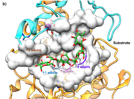
Figure \(\PageIndex{5}\): Surface representation of the active site of HPA (5TD4) https://pdb101.rcsb.org/global-healt...ha-glucosidase. CC-BY-4.0 license. Attribution: David S. Goodsell and the RCSB PDB.
The surface view highlights the deep C-shaped groove into which the substrate, in this case, octaose, is bound. Consistent with protease substrate numbering, the starch substrate is numbered -2, -1, +1, and +2, with cleavage occurring between the -1 and +1 bound alpha-glucose residues. The protein has three domains (orange, blue, and pink). This particular structure contained an active-site mutant (Asp300Asn, D300N). The enzyme has bound calcium and chloride ions. Ca2+ maintains the necessary structure, while Cl-, bound in the C domain, is an allosteric activator.
The octaose binding site is between the A and B domains. Asp197, Glu233, and Asp300 are critical catalytic residues, with Asp 197 acting as a nucleophile to produce a glycosylated intermediate hydrolyzed in the next step. Asp197 and Glu233 act as general acids/bases. We will explore similar mechanisms for the action of beta-amylase (below) and cellulase (in the next chapter section).
Figure \(\PageIndex{6}\) shows an interactive iCn3D modelof starch binding sites on the Human pancreatic alpha-amylase D300N variant complexed with an octaose substrate (5TD4)
.png?revision=1&size=bestfit&width=541&height=341)
 Figure \(\PageIndex{6}\): Starch binding sites on the Human pancreatic alpha-amylase D300N variant complexed with an octaose substrate (5TD4). (Copyright; author via source). Click the image for a popup or use this external link: https://structure.ncbi.nlm.nih.gov/i...W29jf4yAc1JEq9
The domains in the enzyme are color-coded, as in Figure 4. Key active site residues for binding and catalysis are shown as sticks and labeled.
Beta amylase
β-amylase (also called β-1,4-maltosidase) is a key enzyme in the saccharification process, in which starch and cellulose are broken down into monosaccharides. β-amylase is abundant in crops (wheat, barley, soybeans, etc.), other higher plants, bacilli, and fungi. It is used in the production of beer and caramel (malt syrup). As an exo-glycosidase, it cleaves Glc α(1,4) Glc (maltose) units from the nonreducing end of starch. It is called β-amylase since the hydrolysis proceeds with the inversion of configuration at the reducing end of the freed maltose. It can't cleave at α-1,6 branches, so if used alone, this enzyme produces free maltose and large β-limit dextrins. When fruits ripen, the enzyme cleaves starch into the sweet disaccharide maltose. It is also used in seed germination.
Plants have to sprout, which requires energy and free sugars. Maltose is produced on activation of β-amylase during seed germination and sprouting. Although maltose is less sweet than sucrose and fructose, it is used in hard candies because it withstands the heat required in candy production. Malting of grains is accomplished by adding water to sprout them, which leads to the formation of maltose and other sugars. This is followed by drying, after which the malted grains are used as sweeteners in the food industry. Malted grains are used to produce beer, whisky, some baked goods, and other drinks. Barley is the most commonly malted cereal grain.
Huge amounts of amylases are needed for corn ethanol production, and they must withstand the conditions necessary for the industrial production of ethanol. Much effort has been devoted to finding and characterizing microbial β-amylases. We'll describe one, AmyBa, from B. aryabhattai. Figure \(\PageIndex{7}\) shows sequence similarities among various bacterial β-amylases.

Figure \(\PageIndex{7}\): Sequence and structure analysis of AmyBa. . Duan, X., Zhu, Q., Zhang, X. et al. Expression, biochemical, and structural characterization of high-specific-activity β-amylase from Bacillus aryabhattai GEL-09 for application in starch hydrolysis. Microb Cell Fact 20, 182 (2021). https://doi.org/10.1186/s12934-021-01649-5. Creative Commons Attribution 4.0 International License. Creative Commons Attribution 4.0 International License. http://creativecommons.org/licenses/by/4.0/.
Panel A shows multiple sequence alignments of β-amylases. The strictly conserved residues are displayed on a red background, and the highly conserved residues are shown on a yellow background. The secondary structure elements are shown for B. cereus β-amylase (PDB ID: 5BCA). The signal-peptide-cleavage site and two catalytic residues (E) are indicated by black triangles (black inverted triangles). Conservation of the flexible loop motif (HXCGGNVGD) is noted. β-amylase accession numbers are as follows: B. aryabhattai (WP_033580731.1), B. cereus (P36924.2), B. flexus (RIV10038.1), B. firmus (P96513.1), B. circulans (P06547.1), T. thermosulfurigenes (P19584.1).
A comparison of the structures of B. aryabhattai β-amylase with soybean β-amylases is shown in Figure \(\PageIndex{8}\).

Figure \(\PageIndex{8}\) B Three-dimensional molecular model of B. aryabhattai β-amylase (AmyBa). C Superimposition of AmyBa (Blue) and soybean β-amylases (PDB ID: 1Q6C) (gray) and D (PDB ID: 1Q6C) (gray). The C-terminal SBD in microbial β-amylases (box, purple) and the C-terminal loop in plants (box, red). Duan, X, et al., ibid.
The AmyBa has an additional starch-binding domain at the carboxy terminus (Panel B) compared to soybean β-amylases (Panel D).
Since no structures of (AmyBa are publicly available, we present Figure \(\PageIndex{9}\), which shows an interactive iCn3D modelof beta-amylase from Bacillus cereus var. mycoides in complex with maltose (1J0Z)
.png?revision=1&size=bestfit&width=369&height=336)
Figure \(\PageIndex{9}\): Beta-amylase from Bacillus cereus var. mycoides in complex with maltose (1J0Z). (Copyright; author via source).
Click the image for a popup or use this external link: https://structure.ncbi.nlm.nih.gov/i...S2aWbL3z3jPnW8
Like alpha-amylase, β-amylase has an N-terminal catalytic domain with a beta-barrel, a connecting second domain, and a third C-terminal domain, composed primarily of antiparallel β-sheets. Two key catalytic side chains, Glu 172 and Glu 367, are in the beta-barrel.
In Chapter 20.6, we discussed starch synthesis (not its hydrolysis) in detail. We showed that the reaction, which uses an NDP-sugar as a glycan donor, could proceed either with retention or inversion of the anomeric carbon of the donor NDP-sugar. This is illustrated for the reaction of a C1 α-NDP donor monosaccharide with a monosaccharide acceptor to produce the α(1,4) link with retention of configuration or the β(1,4) link with inversion as shown in Figure \(\PageIndex{10}\) below.

Figure \(\PageIndex{10}\): Reaction of a donor NDP-monosaccharide and an acceptor monosaccharide with retention or inversion of configuration at the anomeric carbon of the donor
The same stereochemical outcomes are possible for the hydrolysis of acetal bonds by glycosyl hydrolases. Alpha-amylases cleave the α (1,4) glycosidic bonds to produce shorter dextrins (containing branched glucose units not cleaved by alpha-amylases), and α (1,4) linked glucose oligosaccharides of lengths from 2 glucose units (maltose) up to 7-8. This reaction, hence, proceeds with the retention of configuration. In contrast, beta-amylases cleave starch to produce maltose with an inversion of configuration at the anomeric-reducing end of the maltose. We explore the chemistry of retention and inversion further in the next section on cellulase, which cleaves the β(1,4) acetal link in cellulose. In general, reactions that proceed with inversion react via an SN2 mechanism, similar to the nucleophilic attack on alkyl halides. For the glycosyl transferases that proceed with inversion, the attacking nucleophile on the acceptor is made more nucleophilic by general base catalysis by a deprotonated glutamic or aspartic acid.
Figure \(\PageIndex{11}\) shows the results of in-silico docking studies of a small glycan, maltotetraose, to AmyBa.

Figure \(\PageIndex{11}\): Molecular docking of AmyBa with maltotetraose. The overall structure and substrate binding pocket analysis of AmyBa are shown.
AmyBa displayed very high amylase activity compared to other microbial β-amylases, and its enzymatic activity was much closer to that of sweet potato β-amylase. Molecular dynamics and docking programs can be used to calculate binding energies for substrates. The binding energy and enzymatic activities of bacteria and sweet potato β-amylase were highly correlated, suggesting that the extensive interactions between AmyBa and maltotetraose help drive catalysis by using the energy released upon binding to lower the reaction's activation energy.
Saccharification
To enter glycolysis and fermentation, maltose must be converted to the monosaccharide glucose. The conversion of a polysaccharide to its monomers is called saccharification. To complete the conversion of starch to glucose, another enzyme, glucoamylase (also called amyloglucosidase and γ-amylase), is added. As an exoglucosidase, it cleaves both α (1,4) in amylose, amylopectin, and maltose and α (1,6) branches to form free glucose. It is a member of the glycoside hydrolase family 15 in fungi, glycoside hydrolase family 31 of human maltase-glucoamylase, and glycoside hydrolase family 97 of bacterial forms.
Fermentation
Glucose (C6H12O6) can now enter the glycolytic pathway and continue to ethanol after conversion of pyruvate to acetaldehyde by pyruvate decarboxylase and final conversion of acetaldehyde to ethanol by alcohol dehydrogenase:
C6H12O6 (s) → 2 CH3CH2OH (l) + 2CO2 (g) (anaerobic ethanol biosynthesis)
The yeast Saccharomyces cerevisiae catalyzes this entire pathway.
The final fermentation process yields a 12-15% ethanol solution, which is distilled to form a 95% ethanol/5% water azeotrope. The water is removed by adding zeolites (molecular sieves), which adsorb water but not ethanol.
Life Cycle Analysis of Bioethanol: Is it better than fossil fuels?
We reiterate the promise of bioethanol to address global warming and climate change by presenting again the chemical equations that suggest that its use as a fuel is carbon neutral:
6CO2 (g) + 6H2O (l) → C6H12O6 (s) + 6O2 (photosynthesis)
C6H12O6 (s) → 2 CH3CH2OH (l) + 2CO2 (g) (anaerobic ethanol biosynthesis)
2CH3CH2OH (l) + 6O2 → 4CO2 (g) + 6H2O (g) (combustion of ethanol)
If only these three equations for the production and use of corn bioethanol were the only factors influencing net CO2 emission from bioethanol burning, there would be no controversy about its use. Yet the actual CO2 emissions depend on many more factors hidden from view by these simple equations. A life cycle analysis (LCA) is needed to determine corn ethanol's environmental impact (in this case, net CO2 emissions) across all phases of its life, from cradle to grave, including corn planting and bioethanol use for transportation.
All models must be tested. It's easiest to start with the simplest model. If the data fit the model, great, you're done. If not, new, more expansive models must be developed and tested. Those who vociferously support bioethanol often cite the simple stoichiometry in the three equations to claim that bioethanol is carbon neutral. Most would want a detailed life cycle analysis (LCA) before jumping to an immediate conclusion.
LCAs are very challenging, and data on a global scale is required. Some global-scale measurements have significant uncertainties and are, at best, estimates. A recent study looked at the impact of a specific event, the adoption of the US Renewable Fuel Standards (RFS) that regulate biofuels in the US (which produces about half of all the world's biofuels), on CO2 emissions from the significant increase in corn plant and corn ethanol that followed the adoption of the standard. Using LCA based on a series of economic and environmental metrics, the model shows that bioethanol is not a panacea for CO2 emissions and may be more detrimental than using fossil fuels in vehicles.
The study calculated changes in corn ethanol's carbon intensity after the standards were adopted. Scientists have used other events that led to immediate changes (e.g., 9/11) and 1-2-year changes (e.g., the COVID-19 pandemic) to examine environmental parameters such as CO2 emissions.
Carbon intensity measures how much CO2 or CO2 equivalents are emitted per unit of activity. The unit activity can be kWh of electricity generated, megajoules of energy (MJ) produced by fuel, amount of oil produced, bushels of a particular food produced, or dollars generated (GDP). Ideally, policies should be implemented to decrease carbon intensity. The use of green energy derived from solar and wind lowers carbon intensity. Energy intensity, the total energy production per GDP, is a similar metric.
Figure \(\PageIndex{12}\) shows carbon intensity per GDP per country over the last 30 years (data from Our World in Data).
Figure \(\PageIndex{12}\): Consumption-based carbon intensity from 1990 to 2018. Our World in Data.
The world is generally moving toward more efficient energy production, but our energy consumption is still dramatically increasing.
The LCA model showed that the renewable fuel standards (RFS) policy led to these interrelated outcomes. It:
- increased corn prices by 30% and the prices of other crops by 20%
- increased US corn cultivation by 2.8 Mha (8.7%) and total cropland by 2.1 Mha (2.4%) in the years following policy enactment (2008 to 2016). (1 hectare is an area of a square with 100 meters sides, equivalent to 10,000 m2
- increased annual nationwide fertilizer use by 3 to 8%
- increased water quality degradation by 3 to 5%
- increased emissions from domestic land use changes
According to the study, these combined produced a carbon intensity of corn ethanol that was "no less than gasoline and likely at least 24% higher. "
The changes in the metric are visually described in Figure \(\PageIndex{13}\).

Figure \(\PageIndex{13}\): Changes due to the RFS. (A) Corn planted area. (B) Cropland area. (C) Carbon emissions. (D) Nitrogen applications. (E) Nitrous oxide emissions. (F) Nitrate leaching. (G) Phosphorus applications. (H) Soil erosion. (I) Phosphorus runoff. Positive numbers indicate an increase due to the RFS. Field-level results were aggregated at the county level for enumeration and visualization. Tyler J. Lark et al. PNAS. 119, 2022 (https://doi.org/10.1073/pnas.2101084119) Creative Commons Attribution License 4.0 (CC BY).
Land use changes include farming land that was retired or designated for conservation programs. Tilling additional land releases carbon stored in the soil. Increased farming significantly increased fertilizer production, leading to N2O emissions. In addition, more of the existing cropland was planted with corn. These findings contrast with a USDA study showing that corn ethanol has a 39% lower carbon intensity than gasoline, which was attributed to carbon capture from newly planted crops. However, that study did not account for emissions from land use changes.
LCA can identify production processes that lead to the greatest negative consequences, which, for the sake of this chapter, are greenhouse gas emissions. For example, the LCA for corn ethanol might improve if the CO2 released during anaerobic ethanol biosynthesis could be captured. Outcomes would also change if renewable energy sources were used for stages of production that currently use fossil fuels. These studies also don't account for the hazardous pollutants released during bioethanol production.
This rigorous LCA did not address the moral question of using land that could feed people to produce bioethanol for our ever-bigger vehicles. In addition, opponents of solar energy installations argue that they require so much land that they would displace agricultural uses. What is missing from their argument is the vast amount of land used now for corn ethanol. Farmers planted 90 million acres of corn in 2022 in the US, about 90% of the size of the entire state of California. 44% of that corn went to biofuels, and only 12% went to human consumption. In addition, approximately 44% was used to feed animals for human consumption, an inefficient and unsustainable use of cropland and resources.
Figure \(\PageIndex{13a}\) below shows how little corn is grown in the USA for human consumption.
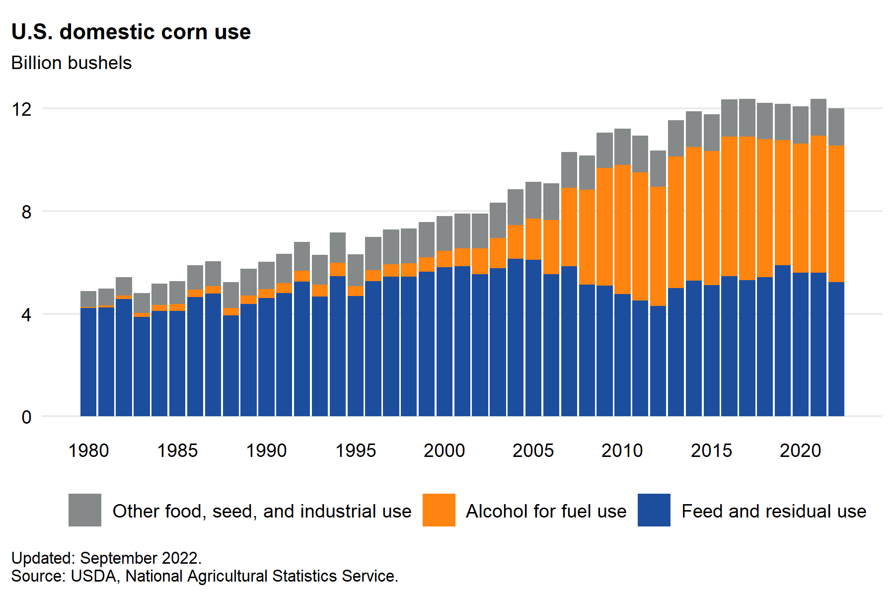
Figure \(\PageIndex{13a}\): Corn and Other Feed Grains - Feed Grains Sector at a Glance. Updated 1/5/2025.
Hannah Ritchie at Our World in Data (the source of many interactive graphs in this chapter) has eloquently and persuasively argued for using solar power to charge electric vehicles rather than corn bioethanol. Here are some conclusions she draws:
- 20 m2 of solar panels produce 1 MWh of electricity per year. This implies that the 25 million hectares of land now used for corn bioethanol (which covers just 10% of our driving fuel) could be covered with solar cells and produce 12,500 TWh. That is about 3 times the USA's annual electricity consumption in 2023.
- Considering just transportation, the main use of biofuels, 1 hectare of solar panels, would allow electric vehicles to travel 3 million km (1.87 million miles). In contrast, 1 hectare of corn for bioethanol will enable cars to travel 22,000 km (13,700 miles).
- People drive approximately 5 trillion km (3.1 trillion miles) annually in the USA. 1.5 million hectares of solar panels would fulfill that energy need (just 6% of the 25 million hectares of land used to produce corn bioethanol, which powers just 10% of our driving needs.
Using agricultural land for crops and solar panels would be a win for all.
Production of sucrose and bioethanol from sugarcane
Like corn, sugar cane, a tropical, perennial grass, is used (mainly in Brazil) to produce ethanol. Sugar cane is a C4 plant with a high ability to fix carbon. It is a perennial that does not need replanting each year, making it a better feedstock than corn for bioethanol production. In 2020, sugar cane was by far the most-produced crop or livestock product in the world (1.87 billion metric tons), followed by corn (1.16 billion metric tons). The production by country for both corn and sugar cane is shown in Figure \(\PageIndex{14}\).
 |
 |
Figure \(\PageIndex{14}\): Corn and sugar cane production by country. Graphs from Our World in Data. https://ourworldindata.org/agricultural-production#
It might surprise you that sugar cane production is so high compared to grain crops that provide nutrition (not just "sweet" calories), but given our addiction to sweet foods, it shouldn't.
Sugar cane is often harvested manually in developing countries. It is then cut, milled, and mixed with water to extract the soluble sucrose (table sugar). Figure \(\PageIndex{15}\) shows the sugar cane components during extraction.

Figure \(\PageIndex{15}\): Components of Sugar Cane (after Larissa Canilha et al. J Biomed Biotechnol. 2012; 2012: 989572. doi: 10.1155/2012/989572
Sucrose is a nonreducing disaccharide (O-α-D-glucopyranosyl-(1,2)-β-D-fructofuranoside). Its structure is shown in Figure \(\PageIndex{16}\).

Figure \(\PageIndex{16}\): Structure of fructose
Sucrose decomposes at 186 °C (367 °F), rather than melting (a feared event for organic chemistry students who wish to record melting temperatures in the lab), to form caramel. Molasses is a viscous liquid product derived from refining sugar cane or sugar beets. It is used as a sweetener for its taste and is also a component of brown sugar. On a sweetness scale, if sucrose is assigned a value of 100, fructose is 140, high fructose corn syrup is 120-160, and glucose is 70-80.
In bioethanol production, sucrose is hydrolyzed by the enzyme invertase into monomeric glucose and fructose. Invertases are activated during the milling and liquefaction of sugarcane, so if sucrose is the desired commercial product, an additional clarification step (heating to 115°C and treating with lime and sulfuric acid) is necessary to prevent hydrolytic cleavage of sucrose.
Bioethanol production from sugar cane sucrose
Bioethanol can be made from either the fibrous lignocellulose remains of the sugar cane, called bagasse, or from water-soluble sucrose. We will describe the production of cellulosic ethanol from field crop stalks, called stover, and leaves, straw, wood chips, and sawdust (all "waste" biomass) in Chapter 31.5. The same principles apply to bioethanol production from bagasse (the solid residue left after sugar cane juice extraction). Note that bagasse is often burned to provide energy for sugar cane processing.
Sugar cane, sugar beets, and sweet sorghum, a C4 plant similar to sugar cane, are also used to produce bioethanol. Sweet sorghum is a very efficient plant for producing biomass through photosynthesis. It grows in temperate and tropical climates, has a short growing period, and is resistant to drought and cold. Its stalks contain free sugars and lignocellulose.
This chapter will focus on bioethanol production from sugar cane sucrose. Again, this is accomplished using yeast (Saccharomyces cerevisiae), which contains the enzyme invertase 2 (beta-fructofuranosidase 2 or Saccharase), which converts sucrose into fructose and glucose, which can enter the glycolytic and fermentation pathways.
Invertase, shown in 1842 to invert the stereochemistry of sugars, was first isolated from yeast in 1860. It has a secreted, glycosylated, homooctameric form and an intracellular form, both of which are products of the same gene. It's a member of Family 32 of the glycoside hydrolases. The structure of the Saccharomyces invertase (SInv) octamer is shown in Figure \(\PageIndex{17}\) below.

Figure \(\PageIndex{17}\): Structure of octameric SInv. M.Angela Sainz-Polo et al. JBC, 288, 9755-9766 (2013). DOI:https://doi.org/10.1074/jbc.M112.446435. Creative Commons Attribution (CC BY 4.0)
Panel a shows views of the SInv octamer in ribbon (left) and solvent-accessible surface (right) representations, with each subunit colored differently.
Panel b shows that the octamer is rotated 90°, illustrating that it can be best described as a tetramer of two different kinds of dimers, AB/CD and EF/HG, which are compared by superimposing subunit F on subunit B in c
Even though all eight subunits in the octamer are identical (58.5K, 512 aa), the quaternary structure of the 8-mer can best be viewed as a tetramer of dimers (i.e., 4 dimers pack to form two packed tetramers giving the octamer). The AB and CD dimers pack in a "closed form" with a narrow active-site pocket, allowing a glycan of 3-4 monomers. The EF and GH dimers pack in an "open form" with a wide active site pocket for longer glycans. Of course, our main interest here is in the binding of sucrose.
Figure \(\PageIndex{18}\) shows an interactive iCn3D modelof Saccharomyces cerevisiae invertase (4EQV)
.png?revision=1&size=bestfit&width=374&height=373)
Figure \(\PageIndex{18}\): Saccharomyces cerevisiae invertase (4EQV). (Copyright; author via source).
Click the image for a popup or use this external link: https://structure.ncbi.nlm.nih.gov/i...ysQW8YSrvPkus9
The color coding of the subunits is the same as shown in the right top image of Panel A, Figure 16 above.
The GH32 enzymes, including invertase, have a catalytic domain consisting of a 5-bladed β-propeller. Each blade has four antiparallel beta-strands. The blades surround an active site enriched in carboxyl side chains.
The "closed" active site of the AB and CD dimers is flanked by Phe 388 and Phe 296, which provide hydrophobic interactions. The "open" form active site of the EF and GH dimers also has a salt bridge between Asp 45 and Lys 385. These are shown in Figure \(\PageIndex{19}\), along with a bound 1-kestose, which is a trisaccharide"sucrose analog" found in vegetables. It consists of a β-D-fructofuranose connected to β-D-fructofuranosyl and α-D-glucopyranosyl residue at the 1- and 2-positions.

Figure \(\PageIndex{19}\): Dimer interface at the active site. The octameric SInv active site interfaces are detailed, keeping the same color pattern as above with one subunit being shown in ribbon representation for clarity. Angela Sainz-Polo et al. JBC, 288, 9755-9766 (2013). DOI:https://doi.org/10.1074/jbc.M112.446435. Creative Commons Attribution (CC BY 4.0)
Panel A shows that the AB/CD dimers have tight interactions between the catalytic and β-sandwich domains. Hydrophobic interactions are observed at the base of the catalytic pocket, mediated by Phe-388 and Phe-296.
Panel b, by contrast, shows that the EF/GH dimers interact only through their β-sandwich domains. In addition, the catalytic pocket contains a new salt bridge between Asp-45 and Lys-385 from the β-sandwich domain, which lines the cavity. A putative 1-kestose molecule is shown in a spherical representation.
The hydrolysis of sucrose by invertase proceeds with the retention of configuration at the anomeric carbon. An active site, Aspartate 22, acts as a nucleophile to form a glycosylated intermediate (fructose-Asp). This is followed by the hydrolysis of the intermediate. An active site, Glutamate 203, acts as a general acid/base. Fructose could also be transferred to another glycan via a transglycosylation reaction. The hydrophobic side chains Phe-388 and Phe-296 line the base of the active site pocket.
Figure \(\PageIndex{20}\) shows an interactive iCn3D modelof the AB dimer of Saccharomyces cerevisiae invertase with key active site residues (4EQV)
.png?revision=1&size=bestfit&width=571&height=374)
Figure \(\PageIndex{20}\): AB dimer of Saccharomyces cerevisiae invertase with key active site residues (4EQV). (Copyright; author via source).
Click the image for a popup or use this external link: https://structure.ncbi.nlm.nih.gov/i...hX9FbxLLip1f97
Figure \(\PageIndex{21}\) shows an interactive iCn3D modelof the EF dimer of Saccharomyces cerevisiae invertase with key active site residues (4EQV). It has an additional salt bridge between Asp-45 and Lys-385.
.png?revision=1&size=bestfit&width=593&height=395)
Figure \(\PageIndex{21}\): EF dimer of Saccharomyces cerevisiae invertase with key active site residues (4EQV). (Copyright; author via source).
Click the image for a popup or use this external link: https://structure.ncbi.nlm.nih.gov/i...Dh33BtT5c8GXK6
Life Cycle Analysis of Sugar Cane Ethanol
Does the production of bioethanol from sugar cane lead to lower net CO2 emissions than bioethanol produced from corn? The answer depends on whether sucrose (first generation) or lignocellulose (second generation) from bagasse is used as the feedstock.
A recent LCA has been performed for the first-generation (sucrose feedstock) production of bioethanol from sugarcane in Ecuador. This sugar-based feedstock has a lower production cost. It requires just grinding and the addition of yeast for fermentation; it does not require a saccharification step.
Figure \(\PageIndex{22}\) shows the various stages and processes used to perform LCA on the bioethanol production from sugar cane sucrose. It's presented to show the complexity of such analyses, so look at the details only if you are especially interested.

Figure \(\PageIndex{22}\): Anhydrous ethanol life cycle system boundaries and main product flow quantification for 2018. Arcentales-Bastidas, D.; Silva, C.; Ramirez, A.D. The Environmental Profile of Ethanol Derived from Sugarcane in Ecuador: A Life Cycle Assessment Including the Effect of Cogeneration of Electricity in a Sugar Industrial Complex. Energies 2022, 15, 5421. https://doi.org/10.3390/en15155421. Creative Commons Attribution (CC BY) license (https://creativecommons.org/licenses/by/4.0/)
The study analyzed four stages, agricultural, milling, distillation, and electricity generation (presumably by burning the byproduct bagasse), for impacts. They defined two functional units:
- 1 ton of sugarcane "at the farm gate” for the agricultural stage;
- 1 L of ethanol "at the plant (factory) gate”.
The key results of the study are as follows:
- The global warming potential (GWP) impact at the "farm gate" was 53.6 kg of carbon dioxide equivalent (kg CO2 equiv) per ton of sugarcane produced. This arises mainly from N2O (34%), a potent greenhouse gas emitted during the process, and from diesel fuel used in agricultural machinery (24%).
- The GWP for 1 L of ethanol produced at the plant gate was 0.60 kg CO2 equiv, with the distillation phase accounting for the largest share.
Before proceeding further, let's explain the key term, global warming potential (GWP), which is widely used in LCA. It accounts for the contributions of other greenhouse gases, such as methane (CH4) and nitrous oxide (N2O), each with unique IR absorption spectra and atmospheric half-lives. The IPCC uses a 100-year time frame for the calculation of the GWP and uses this formula:
CO2 Equivalent kg = CO2 kg + (CH4 kg x 28) + (N2O kg x 265)
\begin{equation}
\mathrm{CO}_2 \text { equivalent } \mathrm{kg}=\mathrm{CO}_2 \mathrm{~kg}+\left(\mathrm{CH}_4 \mathrm{~kg} \times 28\right)+\left(\mathrm{N}_2 \mathrm{O} ~k g \times 265\right)
\end{equation}
- CO2 has a GWP of 1 by definition since it is the reference. Its time frame in the atmosphere (100s to 1000 years) doesn't matter since it is the reference.
- CH4 has a GWP of around 27-30 over 100 years, reflecting its higher IR absorbance but lower lifetime (around 12 years).
- N2O has a GWP of around 265-273 over a 100-year timescale and a lifetime of around 109 years.
The equation can be amended to account for other greenhouse gases emitted from manufacturing and refrigerant use. These include Freon-12 (Dichlorodifluoromethane) (CFC-12), with a lifetime of 100 years and a GWP100 of 10,200, and SF6 (used in the electricity industry to keep networks running safely and reliably), with a lifetime of 3200 years and a GWP00 of 23,500!
N2O (laughing gas) is an overlooked source of greenhouse gases, accounting for about 7% of the warming effect of long-lived, high-GWP gases. Agricultural practices lead to about 65% of its total emissions. It is a component of the soil and atmosphere nitrogen cycle. In soil, its concentration depends on soil microbes that engage in nitrification and denitrification processes. These depend on the amount of fixed nitrogen, oxygen levels, and metabolically available carbon sources. The nitrification reaction, which occurs in aerated, moist soils, involves the oxidation of NH3↔NH4+ to NO2 and NO3-, with some N2O produced. The primary source of N2O occurs under anaerobic conditions. These general reactions are shown below.
- Nitrification (aerobic, oxidation): N2 → (NH3 ↔ NH4+) → NO2 → NO3-
- Denitrification (anaerobic, reduction): NO3− → NO2− → NO → N2O → N2
In anaerobic environments, NO serves as an electron acceptor during microbial respiration. N2O is produced when excess nitrogen is available (beyond the needs of plants and microorganisms), so excessive use of fertilizers and manure increases its production. Nitrifying and denitrifying bacteria are most active in producing N2O in environments with abundant N relative to assimilatory demands by other microorganisms or plants (Firestone and Davidson, 1989), as is often the case following soil amendment with fertilizers, manure, or crop residues. Physical soil processing (such as tillage) also affects N2O emissions by introducing crop residues into the soil, altering soil particle size and surface area, and altering soil porosity. These affect soil substrate/product availability and the rates of aqueous and gas diffusion.
Let's use dimensional analysis from introductory chemistry to convert the GWP from the farm gate/agricultural stage (53.6 kg CO2 equiv/ton of sugar cane) to kg CO2 equiv/1L of ethanol (EtOH) so we can add it to the GWP from the plant gate, which is expressed in kg CO2 equiv/L ethanol produced. The dimensional conversion is shown in Table \(\PageIndex{2}\) below.
| 53.6 kg CO2 equiv | 1 ton SC | 1 L Juice | = | 0.1 kg CO2 equiv |
| 1 ton SC | 800 L juice | 0.7 L EtOH | 1 L EtOH produced |
Table \(\PageIndex{2}\): Conversion of 53.6 Kg CO2 equiv/ton of sugar cane from the farm gate (left-hand column) to 0.1 Kg CO2 equiv/1L of ethanol (EtOH).
Now, add this to the reported 0.60 kg CO2 equiv/1 L of ethanol from the plant (factor) gate, and you will get a total of 0.7 kg CO2 equiv/1 L of ethanol produced from sugar cane. This compares with a reported value of 2.3 kg CO2 equiv/1 L of gasoline produced, so, based on this study, sugar cane-derived bioethanol is significantly better, as its manufacturing emits less CO2 equiv than gasoline manufacturing.
But remember that ethanol is partially oxidized and produces less energy per unit of mass on combustion. Burning 1 L of gasoline releases 33.6 MJ of energy, while 21.2 MJ is released on burning ethanol, so we should multiply the 0.7 kg CO2 equiv /1 L of ethanol by 33.6/21.2 = 1.6 to give a normalized carbon intensity = 0.95. This uses the equivalent amount of ethanol (1.6 L) to give the same energy as 1 L of gasoline. Still, burning sugar to produce bioethanol is better than burning gasoline on a CO2-equivalent basis.
The promise of bioethanol is based on the notion that 1 C atom is used to produce it and 1 C atom is released during its combustion, as illustrated in the equations we saw above (and presented again below).
Eq 1: 6CO2 (g) + 6H2O (l) → C6H12O6 (s) + 6O2 (photosynthesis)
Eq 2: C6H12O6 (s) → 2 CH3CH2OH (l) + 2CO2 (g) (anaerobic ethanol biosynthesis)
Eq 3: 2CH3CH2OH (l) + 6O2 → 4CO2 (g) + 6H2O (g) (combustion of ethanol)
Now add to this series of net-zero CO2 reactions the release of CO2 from the manufacture of bioethanol, and you can see that the notion of net 0 for biofuels is misleading. Based on the analyses above, burning bioethanol from sugar cane produces significantly less CO2 equiv than gasoline, but it's nowhere near net 0. Biofuel use can play a big role in reducing emissions when it replaces gasoline, but it must be coupled with other ways to reduce emissions (such as solar and wind) to achieve the magnitude of reductions we need. It also appears the jury is still out on the environmental benefits of corn bioethanol.
The LCA analysis described above assesses the global warming potential of using sugarcane sucrose for bioethanol production. However, bioethanol production from sugar cane juice has other negative impacts, as listed below in Table \(\PageIndex{4}\).
| Impact Category | Characterization Factor | Reference Unit |
|---|---|---|
| Climate change | Climate change—GWP100 | kg CO2eq. |
| Freshwater eutrophication | Freshwater eutrophication potential—FEP | kg Peq. |
| Marine eutrophication | Marine eutrophication potential—MEP | kg Neq. |
| Abiotic depletion | Metal depletion—MDP | kg Feeq. |
| Photooxidant formation | Photochemical oxidant formation potential—POFP | kg NMVOCeq. |
| Particulate matter emissions | Particulate matter formation potential—PMFP | kg PM10eq. |
| Terrestrial acidification | Terrestrial acidification potential—TAP100 | kg SO2eq. |
Biofuels or Solar?
The case for devoting so much land to biofuel production is weak, as outlined above. Even if it is marginally better in net emissions compared to using fossil fuels, that does not account for what economists call opportunity cost, the cost of things not done or considered in the decision to use biofuels to address climate change. What benefits are we missing when choosing one options, biofuels, versus another (solar for example).
The world is clearly accelerating its investment in biofuels, as indicated in Figure \(\PageIndex{23}\) below.
Figure \(\PageIndex{23}\): Biofuel energy production since 1990. Hannah Ritchie and Pablo Rosado (2026) - “Putting solar panels on land used for biofuels would produce enough electricity for all cars and trucks to go electric”. Published online at OurWorld. inData.org. Retrieved from: 'https://archive.ourworldindata.org/2...-vehicles.html' [Online Resource] (archived on January 23, 2026
This graph includes both ethanol and biodiesel (from oil crops such as soybeans and palm oil, discussed in a future section) generated not only from corn (the US) but also from sugarcane (Brazil, also discussed in a future section). What if the same equivalent land use presently devoted to biofuel crop production were used for solar panel installation? Presently, about 32 million hectares (about 124K square miles, the land area of Poland) are used to produce biofuels (1400 TWh, which power 4% of our transport). If they were instead covered with solar panels, 23 times as much electrical energy (32,000 TWh/yr) could be produced each year (Ritchie and Rosado, ibid.). This area of solar cells would not be installed in one place but would be distributed around the world and could, in part, be colocated on land used for agriculture. The emerging field of agrivoltaics does exactly that.
Ritchie and Rosado note that only 1% of the sun's energy is used to produce biomass, and that even more is effectively lost when that biomass is turned into fuel. In contrast, modern photocells convert around 22% of the sun's energy directly into electrical energy. That could help decarbonize the transport industry as we move from internal combustion engines to electric vehicles.
Summary
(Summary written by Claude, Anthropic)
This chapter examines the biochemistry, industrial processes, and environmental impact of first-generation bioethanol production from corn and sugar cane — the dominant biofuels globally — within the broader context of climate change mitigation.
Energy context. Ethanol contains one oxygen atom in a two-carbon molecule, making it partially oxidized and consequently less energy-dense than gasoline: it releases ~29.7 kJ/g versus ~47.9 kJ/g for octane, delivering about 63% of gasoline's energy by mass and 70% by volume. The US produced 16 billion gallons of fuel ethanol at peak production in 2018 — about one-tenth of annual US gasoline consumption — with the US and Brazil together accounting for ~85% of global fuel ethanol. The theoretical case for bioethanol rests on three coupled reactions: photosynthesis fixes atmospheric CO₂ into glucose, fermentation converts glucose to ethanol plus CO₂, and combustion returns CO₂ to the atmosphere. This stoichiometric argument suggests net-zero carbon emissions, but a full life cycle analysis reveals a far more complex picture.
Corn starch hydrolysis: enzyme biochemistry. Corn starch — an α(1,4) glucose polymer with α(1,6) branches — must be hydrolyzed to free glucose before fermentation. This requires three enzyme types working in sequence. α-Amylase (endoglucosidase) cleaves internal α(1,4) bonds to produce short dextrins and maltooligosaccharides, proceeding with retention of anomeric configuration via a covalent glycosyl-enzyme intermediate; Asp197 acts as the nucleophile and Glu233 as the general acid/base, with Ca²⁺ maintaining structure and Cl⁻ acting as an allosteric activator. β-Amylase (exoglucosidase) cleaves successive maltose units from non-reducing ends with inversion of anomeric configuration — an SN2-like mechanism using two glutamate residues — but cannot cleave α(1,6) branch points, leaving large β-limit dextrins. Glucoamylase (γ-amylase) completes saccharification by cleaving both α(1,4) and α(1,6) bonds to release free glucose. Industrial microbial β-amylases, such as AmyBa from Bacillus aryabhattai, offer high specific activity and an additional C-terminal starch-binding domain; molecular docking studies show that binding energy correlates strongly with enzymatic activity, supporting an induced-fit mechanism.
Sugar cane and invertase biochemistry. Sugar cane — a C4 perennial grass and the world's most-produced crop (1.87 billion metric tons in 2020) — is primarily used in Brazil for bioethanol. Its sucrose (a non-reducing α(1,2)-linked glucose-fructose disaccharide) is hydrolyzed by invertase (β-fructofuranosidase) with retention of configuration. S. cerevisiae invertase is an octamer best described as a tetramer of dimers: the AB/CD dimers adopt a "closed" active-site configuration stabilized by hydrophobic Phe-388 and Phe-296 interactions, while the EF/GH dimers adopt an "open" configuration with an additional Asp45–Lys385 salt bridge. The catalytic mechanism involves Asp22 as a nucleophile forming a fructose-enzyme intermediate, and Glu203 as a general acid/base. Sugar cane has significant advantages over corn: it requires no saccharification step (sucrose is directly fermentable), does not need annual replanting, and has higher photosynthetic efficiency through C4 metabolism.
Life cycle analysis of corn ethanol. The Lark et al. (2022) study used the adoption of the US Renewable Fuel Standards (2005) as a natural experiment to assess the full environmental impact of expanding corn ethanol production. The results were sobering: the policy increased corn cultivation by 2.8 million hectares, raised fertilizer use by 3–8%, increased N₂O emissions (a GWP₁₀₀ of 265), degraded water quality by 3–5%, and released soil carbon through land-use change. The combined carbon intensity of corn ethanol was found to be "no less than gasoline and likely at least 24% higher." These findings directly contradict a USDA study claiming 39% lower carbon intensity — the discrepancy arising from the USDA study's failure to account for land-use change emissions. The moral question of using food cropland for fuel (44% of US corn goes to biofuels; only 12% to direct human consumption) adds further weight to the critique.
Life cycle analysis of sugar cane ethanol. An Ecuadorian LCA of sugar cane sucrose-based bioethanol found a farm-gate GWP of 53.6 kg CO₂ equiv/ton of sugarcane, dominated by N₂O emissions (34%) from fertilizer use and diesel combustion (24%). Converting to comparable units (0.1 kg CO₂ equiv/L ethanol from the farm gate plus 0.60 kg CO₂ equiv/L from the plant gate = 0.70 kg CO₂ equiv/L) and normalizing for the lower energy density of ethanol (×1.6 to match gasoline's energy output) gives a carbon intensity of ~0.95 kg CO₂ equiv/L-gasoline-equivalent — substantially lower than gasoline's 2.3 kg CO₂ equiv/L. Sugar cane ethanol is therefore significantly better than gasoline on a lifecycle basis, but far from carbon-neutral. N₂O — produced by nitrifying bacteria under aerobic conditions and denitrifying bacteria under anaerobic conditions whenever excess fixed nitrogen is present — is a major and often underappreciated contributor to the GWP of any nitrogen-fertilizer-intensive crop.
Biofuels versus solar: the opportunity cost. The most powerful challenge to large-scale biofuel expansion comes from land-use efficiency comparisons. Approximately 32 million hectares currently devoted to biofuel crops produce ~1,400 TWh/year of energy, powering ~4% of global transport. If covered with modern photovoltaic panels (~22% efficiency vs. ~1% for biomass), the same land area would generate ~32,000 TWh/year — 23 times more energy. Per hectare, solar enables electric vehicles to travel ~3 million km versus ~22,000 km from corn ethanol. Hannah Ritchie's analysis concludes that 1.5 million hectares of solar panels — just 6% of current US corn bioethanol land — could power all US passenger driving. The concept of opportunity cost is central: every hectare devoted to biofuels is a hectare unavailable for vastly more efficient solar energy production, food crops, or carbon-sequestering natural ecosystems. Biofuels can play a transitional role in reducing emissions compared to fossil fuels in hard-to-electrify sectors, but the emerging consensus is that solar electrification of transportation is far superior to bioethanol as a climate mitigation strategy.