
3: Use of Isotope Analysis in Measuring Climate Change
- Page ID
- 34458
\( \newcommand{\vecs}[1]{\overset { \scriptstyle \rightharpoonup} {\mathbf{#1}} } \)
\( \newcommand{\vecd}[1]{\overset{-\!-\!\rightharpoonup}{\vphantom{a}\smash {#1}}} \)
\( \newcommand{\dsum}{\displaystyle\sum\limits} \)
\( \newcommand{\dint}{\displaystyle\int\limits} \)
\( \newcommand{\dlim}{\displaystyle\lim\limits} \)
\( \newcommand{\id}{\mathrm{id}}\) \( \newcommand{\Span}{\mathrm{span}}\)
( \newcommand{\kernel}{\mathrm{null}\,}\) \( \newcommand{\range}{\mathrm{range}\,}\)
\( \newcommand{\RealPart}{\mathrm{Re}}\) \( \newcommand{\ImaginaryPart}{\mathrm{Im}}\)
\( \newcommand{\Argument}{\mathrm{Arg}}\) \( \newcommand{\norm}[1]{\| #1 \|}\)
\( \newcommand{\inner}[2]{\langle #1, #2 \rangle}\)
\( \newcommand{\Span}{\mathrm{span}}\)
\( \newcommand{\id}{\mathrm{id}}\)
\( \newcommand{\Span}{\mathrm{span}}\)
\( \newcommand{\kernel}{\mathrm{null}\,}\)
\( \newcommand{\range}{\mathrm{range}\,}\)
\( \newcommand{\RealPart}{\mathrm{Re}}\)
\( \newcommand{\ImaginaryPart}{\mathrm{Im}}\)
\( \newcommand{\Argument}{\mathrm{Arg}}\)
\( \newcommand{\norm}[1]{\| #1 \|}\)
\( \newcommand{\inner}[2]{\langle #1, #2 \rangle}\)
\( \newcommand{\Span}{\mathrm{span}}\) \( \newcommand{\AA}{\unicode[.8,0]{x212B}}\)
\( \newcommand{\vectorA}[1]{\vec{#1}} % arrow\)
\( \newcommand{\vectorAt}[1]{\vec{\text{#1}}} % arrow\)
\( \newcommand{\vectorB}[1]{\overset { \scriptstyle \rightharpoonup} {\mathbf{#1}} } \)
\( \newcommand{\vectorC}[1]{\textbf{#1}} \)
\( \newcommand{\vectorD}[1]{\overrightarrow{#1}} \)
\( \newcommand{\vectorDt}[1]{\overrightarrow{\text{#1}}} \)
\( \newcommand{\vectE}[1]{\overset{-\!-\!\rightharpoonup}{\vphantom{a}\smash{\mathbf {#1}}}} \)
\( \newcommand{\vecs}[1]{\overset { \scriptstyle \rightharpoonup} {\mathbf{#1}} } \)
\(\newcommand{\longvect}{\overrightarrow}\)
\( \newcommand{\vecd}[1]{\overset{-\!-\!\rightharpoonup}{\vphantom{a}\smash {#1}}} \)
\(\newcommand{\avec}{\mathbf a}\) \(\newcommand{\bvec}{\mathbf b}\) \(\newcommand{\cvec}{\mathbf c}\) \(\newcommand{\dvec}{\mathbf d}\) \(\newcommand{\dtil}{\widetilde{\mathbf d}}\) \(\newcommand{\evec}{\mathbf e}\) \(\newcommand{\fvec}{\mathbf f}\) \(\newcommand{\nvec}{\mathbf n}\) \(\newcommand{\pvec}{\mathbf p}\) \(\newcommand{\qvec}{\mathbf q}\) \(\newcommand{\svec}{\mathbf s}\) \(\newcommand{\tvec}{\mathbf t}\) \(\newcommand{\uvec}{\mathbf u}\) \(\newcommand{\vvec}{\mathbf v}\) \(\newcommand{\wvec}{\mathbf w}\) \(\newcommand{\xvec}{\mathbf x}\) \(\newcommand{\yvec}{\mathbf y}\) \(\newcommand{\zvec}{\mathbf z}\) \(\newcommand{\rvec}{\mathbf r}\) \(\newcommand{\mvec}{\mathbf m}\) \(\newcommand{\zerovec}{\mathbf 0}\) \(\newcommand{\onevec}{\mathbf 1}\) \(\newcommand{\real}{\mathbb R}\) \(\newcommand{\twovec}[2]{\left[\begin{array}{r}#1 \\ #2 \end{array}\right]}\) \(\newcommand{\ctwovec}[2]{\left[\begin{array}{c}#1 \\ #2 \end{array}\right]}\) \(\newcommand{\threevec}[3]{\left[\begin{array}{r}#1 \\ #2 \\ #3 \end{array}\right]}\) \(\newcommand{\cthreevec}[3]{\left[\begin{array}{c}#1 \\ #2 \\ #3 \end{array}\right]}\) \(\newcommand{\fourvec}[4]{\left[\begin{array}{r}#1 \\ #2 \\ #3 \\ #4 \end{array}\right]}\) \(\newcommand{\cfourvec}[4]{\left[\begin{array}{c}#1 \\ #2 \\ #3 \\ #4 \end{array}\right]}\) \(\newcommand{\fivevec}[5]{\left[\begin{array}{r}#1 \\ #2 \\ #3 \\ #4 \\ #5 \\ \end{array}\right]}\) \(\newcommand{\cfivevec}[5]{\left[\begin{array}{c}#1 \\ #2 \\ #3 \\ #4 \\ #5 \\ \end{array}\right]}\) \(\newcommand{\mattwo}[4]{\left[\begin{array}{rr}#1 \amp #2 \\ #3 \amp #4 \\ \end{array}\right]}\) \(\newcommand{\laspan}[1]{\text{Span}\{#1\}}\) \(\newcommand{\bcal}{\cal B}\) \(\newcommand{\ccal}{\cal C}\) \(\newcommand{\scal}{\cal S}\) \(\newcommand{\wcal}{\cal W}\) \(\newcommand{\ecal}{\cal E}\) \(\newcommand{\coords}[2]{\left\{#1\right\}_{#2}}\) \(\newcommand{\gray}[1]{\color{gray}{#1}}\) \(\newcommand{\lgray}[1]{\color{lightgray}{#1}}\) \(\newcommand{\rank}{\operatorname{rank}}\) \(\newcommand{\row}{\text{Row}}\) \(\newcommand{\col}{\text{Col}}\) \(\renewcommand{\row}{\text{Row}}\) \(\newcommand{\nul}{\text{Nul}}\) \(\newcommand{\var}{\text{Var}}\) \(\newcommand{\corr}{\text{corr}}\) \(\newcommand{\len}[1]{\left|#1\right|}\) \(\newcommand{\bbar}{\overline{\bvec}}\) \(\newcommand{\bhat}{\widehat{\bvec}}\) \(\newcommand{\bperp}{\bvec^\perp}\) \(\newcommand{\xhat}{\widehat{\xvec}}\) \(\newcommand{\vhat}{\widehat{\vvec}}\) \(\newcommand{\uhat}{\widehat{\uvec}}\) \(\newcommand{\what}{\widehat{\wvec}}\) \(\newcommand{\Sighat}{\widehat{\Sigma}}\) \(\newcommand{\lt}{<}\) \(\newcommand{\gt}{>}\) \(\newcommand{\amp}{&}\) \(\definecolor{fillinmathshade}{gray}{0.9}\)Search Fundamentals of Biochemistry
-
Reconstructing Paleoclimate Records:
- Understand how scientists use isotope analyses of ice cores and ocean sediment cores to reconstruct CO₂ and temperature values over millions of years.
- Explain the importance of long-term climate records for validating current climate models and understanding the relationship between atmospheric CO₂ and temperature.
-
Fundamentals of Isotope Effects:
- Define key concepts, such as isotopes, isotope fractionation, and δ (delta) values (e.g., δ¹⁸O, δ¹³C), and their significance in climate science.
- Describe how isotope partitioning in water and biomolecules involves both equilibrium and non-equilibrium processes, analogous to biochemical reaction pathways.
-
Proxy Data and Calibration Techniques:
- Identify various proxies (e.g., tree rings, foraminifera shells, coral growth bands) used to infer past temperatures and CO₂ levels, and discuss their calibration using modern measurements.
- Compare theoretical calibration equations (e.g., the Kim and O’Neil equation) with empirical data from cultured organisms to inform temperature reconstruction.
-
Chemical Reactions and Fractionation Processes:
- Analyze the chemical reactions involved in the incorporation of heavy isotopes (like ¹⁸O) into calcium carbonate and how these processes are influenced by temperature, salinity, and pH.
- Evaluate the role of equilibrium and kinetic controls in isotope fractionation during calcite formation in marine organisms.
-
Interdisciplinary Integration:
- Connect isotope effects in biochemistry with their application in climate science, demonstrating how principles from organic, analytical, and physical chemistry contribute to understanding Earth's climate history.
- Discuss how a deep understanding of isotopic partitioning enhances insights into both metabolic pathways and large-scale environmental changes.
-
Methodological Rigor and Data Interpretation:
- Appreciate the intellectual rigor and endurance required to obtain, interpret, and model isotopic data over geological timescales.
- Critically assess the strengths, limitations, and uncertainties in the use of proxies for reconstructing past CO₂ concentrations and temperatures.
-
Application of Isotope Ratios in Climate Models:
- Understand how isotope ratios of oxygen (¹⁸O/¹⁶O) in water and carbonates are used to infer temperature changes and ice volume variations over time.
- Explain the significance of Rayleigh distillation and other fractionation processes in determining δ¹⁸O values in different environmental settings.
-
Biological Contributions to Proxy Records:
- Describe the roles of ocean microorganisms—such as planktonic and benthic foraminifera, diatoms, and other phytoplankton—in contributing to sedimentary records used for isotope analysis.
- Analyze how the biological processes that form these shells impact the isotopic composition and thus the interpretation of paleotemperature data.
-
Linking Past and Present:
- Compare proxy-derived temperature records with direct observations from modern instruments to validate reconstruction methods.
- Explore how understanding past climate variability can inform predictions about future climate changes and guide mitigation strategies.
-
Ethical and Scientific Responsibility:
- Recognize the ethical importance of rigorous scientific methods in building reliable climate models that inform policy and societal responses to climate change.
- Discuss the role of scientific integrity in ensuring that proxy data and isotope analyses accurately represent Earth's climatic history, thereby building public trust in climate science.
These learning goals aim to integrate biochemical principles with paleoclimate reconstruction techniques, enabling biochemistry majors to appreciate the interdisciplinary methods used to understand Earth's climate history and their relevance to contemporary environmental challenges.
This chapter will explore how to reconstruct CO2 and temperature values across millions of years. It is truly a remarkable, if not awe-inspiring, achievement that shows the intellectual rigor and endurance scientists employ to obtain, interpret, and model data. The graphs of CO2 vs. temperature across such a vast swath of time shown in the previous chapter section were obtained from analyses of oxygen and carbon isotopes in chemical species from ice and ocean-floor sediments. Interpreting the isotope data requires understanding the link between individual and linked chemical and biochemical reactions. So, we have to deeply dive into isotopes and their use.
- Isotopes and their effects are critical to understanding the structure and activity of biochemical reactions and to climate science.
- Isotope partitioning into water and biomolecules involves both equilibrium and nonequilibrium reactions and processes, similar to linked biochemical reactions and pathways.
- The study and application of isotope effects can integrate and expand learning from previous science courses.
In more global terms
- We must assess the quality and robustness of our data and models to support our understanding of biochemistry and climate change.
- Scientific and ethical rigor are essential for pursuing knowledge, explanations, and solutions in biochemistry and climate change. It is necessary to trust our experts and believe in their findings.
Absolute and proxy measurements for CO2 and temperature
It's simple to see how CO2 levels over the last 800,000 years have been determined from ice cores, since ancient air is trapped in bubbles in them. The bubbles can be liberated by melting/shattering and analyzed. However, how can we infer temperature changes or actual temperature from ice core samples and both CO2 and temperature from ocean sediment cores? Scientists use "proxies" to determine temperature, as modern thermometers and temperature scales were invented only recently (in the early and mid-1700s by Fahrenheit and Celsius). These proxies include tree rings, growth bands in coral, pollens found in core samples, and calcite shells from marine organisms found in lake and ocean sediments. The organisms include certain types of algae, phytoplankton like dinoflagellates and diatoms, and foraminifera (single-celled protozoans with shells).
From a more chemical perspective, analyses of the isotopic composition of ice, using the 18O/16O ratio in water, and of marine sediments, using the ratio of 18O/16O and 13C/12C in carbonate-containing shells, have proved critical in determining temperatures back millions of years. Even molecules in leaf waxes (as discussed in Chapter 31.1) can be used. Isotope analyses of diatoms (with silicate shells) in lake sediments are also useful.
The analysis of proxies is quite complicated, as many factors contribute to the measurements derived from proxy use. Take tree rings as an example. The width of a given ring depends not only on temperature but also on precipitation. Each proxy must be calibrated using alternative data, such as tree-ring data. Proxy data from ice cores extends back a few million years, while marine sediment data extends back as far as 100 million years. Isotope analysis in rocks formed from marine or land sediments can go back billions of years. Recently collected proxy data (tree rings) can be compared with actual temperature measurements from the same period. The calibration relationships can then be used for past samples. Alternatively, proxy data can be taken across many different places and temperatures to develop calibration constants, an approach useful for pollen analysis. To calibrate past data, organisms could also be cultured under different temperatures, nutrient conditions, and CO2 levels. Statistically, it is best to combine multiple proxies to reconstruct past temperatures. Proxy data sets are available for over 10,000 sites worldwide. Figure \(\PageIndex{1}\) below links to sites compiled by Carbon Brief, where databases with information about each study are available.
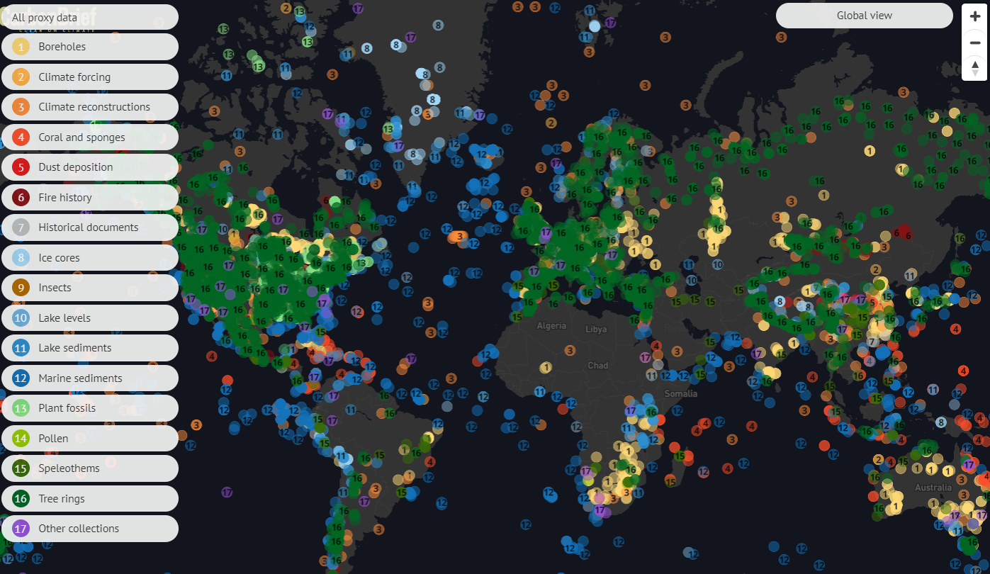
Figure \(\PageIndex{1}\): Map of over 10,000 proxy data studies and sites. Robert McSweeney, Zeke Hausfather, and Tom Prater. https://interactive.carbonbrief.org/...-distant-past/
Most people might care little about climate change millions of years ago. The value of understanding climate change in the past is, in part, to build confidence in the data, methods of analysis, and climate models to better understand the relationship between CO2 and temperature. Some, particularly the PAGES 2k Consortium, focus on the last 2000 years of the Common Era. Figure \(\PageIndex{2}\) shows global mean temperatures obtained from proxy data (yrs 0 - 2000) and direct observations (through the use of thermometer and satellite measurements) since around 1850.
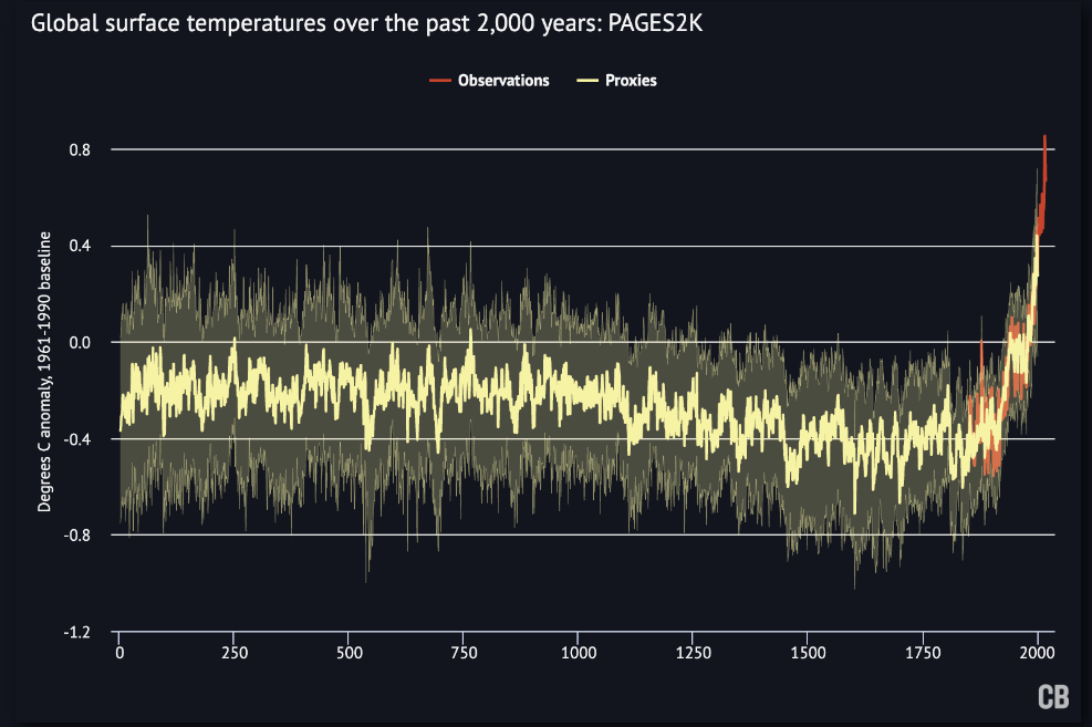
Figure \(\PageIndex{2}\): Global mean surface temperature reconstruction (yellow line) and uncertainties (yellow range) for the years 0-2000 period from the PAGES 2k Consortium along with observations from Cowtan and Way from 1850-2017. Data available in the NOAA Paleoclimate Archive.
Note the overlap of proxy measurements and direct observations of temperatures since around 1850.
Ocean Microorganisms
Biochemistry students come from many backgrounds, but not all have a strong background in biology. Let's look at a few relevant topics in this chapter to help with that and to develop a sense of wonder about the microorganisms that inhabit the oceans and play such a key part in the biosphere. These descriptions are probably new for those with a "chemistry-centric" focus.
Plankton
The word plankton derives from a Greek word meaning drifter or wanderer. There are two main types. One is zooplankton, which are not plants but rather microscopic animals and protozoans. They are heterotrophs that don't synthesize their food. Most have calcite shells. The other is phytoplankton, autotrophic organisms that use photosynthesis to produce food. Hence, they are carbon "capturers", key players in the carbon cycle in maintaining atmospheric CO2 and producing O2. The phytoplankton broadly includes algae (protists), cyanobacteria (also known as blue-green algae), and dinoflagellates, which also fit into other groups. Here are some examples. Also, remember that protists are eukaryotic organisms, not animals, plants, or fungi.
| Type of plankton | Examples |
|---|---|
| Zooplankton (heterotrophs) |
Benthic foraminiferans, which live mostly on the sea bottom and in sediment, capture carbon indirectly in the carbon cycle through carbonate in their shells. Planktonic foraminifera, which live near the surface but are found buried in ocean sediments after their death Dinoflagellates that don't photosynthesize are small animals, including tiny fish and crustaceans such as krill and jellyfish. Radiolarians, single-cell protozoans that have calcium silicate shells |
| Phytoplankton (autotrophs, primary producers) |
Diatoms Photosynthesizing dinoflagellates Blue-green algae, which are prokaryotic bacteria Green algae, photosynthetic eukaryotic protists. Some foraminifera that live near the surface water and can photosynthesize |
Zooplankton
Existing shells in marine sediments from foraminifera have been critical for dating studies and for determining CO2 levels and temperatures over millions of years. Two major types are benthic foraminifera (which live at the sea bottom and in sediment) and a smaller group of planktonic foraminifera, which live near the surface. They are heterotrophs, but when they ingest small autotrophic phytoplankton, some can retain and sequester their chloroplasts, which can continue photosynthesis for a while. Figures \(\PageIndex{3-5}\) below show examples of zooplankton that have been important in climate studies.
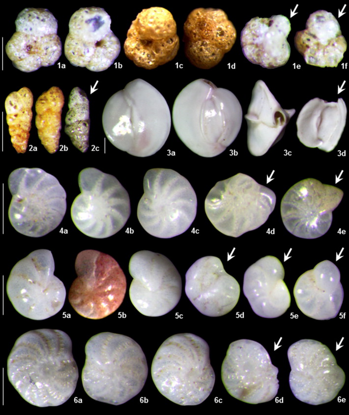
Figures \(\PageIndex{3}\) above: Benthic foraminifera:
Live mostly at the sea bottom and in sediment); capture carbon indirectly through the carbon cycle by incorporating CO32- into their shells. Living benthic foraminifera in the Bohai Sea, showing normal specimens and abnormal individuals (indicated by arrows).

Figures \(\PageIndex{4}\) above: Planktonic foraminifera
They live near the surface but are buried in ocean sediments after death. (a–h) Nano-CT scan of planktonic foraminifera specimens with a color map of test thickness, warm colors indicating areas of relatively thicker shell; (a,b) Globigerinoides ruber (Tara), (c) Globigerina bulloides (Tara), (d) Neogloboquadrina dutertrei (Tara), (e) G. ruber (Challenger), (f) Trilobatus trilobus (Challenger), (g) N. acostaensis (Challenger), (h) N. dutertrei (Challenger); (i–p) SEM images of selected planktonic foraminifera specimens; (i) T. trilobus (Tara), (j) G. ruber (Tara), (k) G. ruber (Challenger), (l) G. bulloides (Challenger), (m,n) G. ruber test cracked to reveal wall texture (Tara), (o,p) G. ruber test cracked to reveal wall texture (Challenger).
Figures \(\PageIndex{5}\) Above: Radiolaria .single-cell protists that secrete silica
Figures \(\PageIndex{3-5}\): Examples of zooplankton. Benthic foraminifera: https://commons.wikimedia.org/wiki/F...raminifera.p; Planktonic foraminifera: Creative Commons Attribution 4.0 International License. Fox, L., Stukins, S., Hill, T. et al. Quantifying the Effect of Anthropogenic Climate Change on Calcifying Plankton. Sci Rep 10, 1620 (2020). https://doi.org/10.1038/s41598-020-58501-w. http://creativecommons.org/licenses/by/4.0/.; Radilaria: https://commons.wikimedia.org/wiki/F...ria-sp2_hg.jpg
Phytoplankton
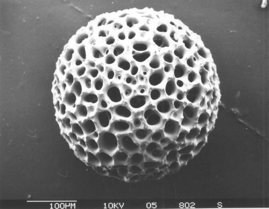
Phytoplankton are microscopic plants that use photosynthesis, capture CO2, and produce O2. Hence, they are primary autotrophs. We will consider three types: diatoms, photosynthetic dinoflagellates, and coccolithophores. Diatoms and photosynthetic dinoflagellates are the major ones and are prey for the zooplankton. They are described in Figures \(\PageIndex{6-8}\) below.
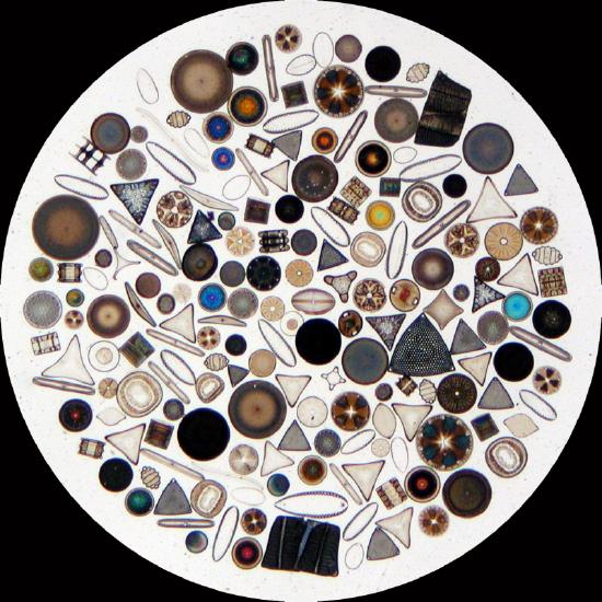
Figures \(\PageIndex{6}\) Above: diatoms
Single-celled eukaryotic algae are surrounded by a silica shell (test). These can reach 1 mm in diameter and take various shapes. Some can form multicellular chains. They engage in high-efficiency photosynthesis, resulting in carbohydrate synthesis. They are found in coastal and cold-water habitats that are rich in nutrients.
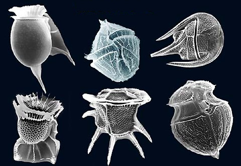
Figures \(\PageIndex{7}\) Above: photosynthetic dinoflagellates
Algae with a single shell. They are smaller than diatoms. Most have two flagella for motion. They have a cellulose shell, which degrades upon death. Hence, they don't have shells that enter the sediment. Some are nonphotosynthetic and are considered zooplankton.
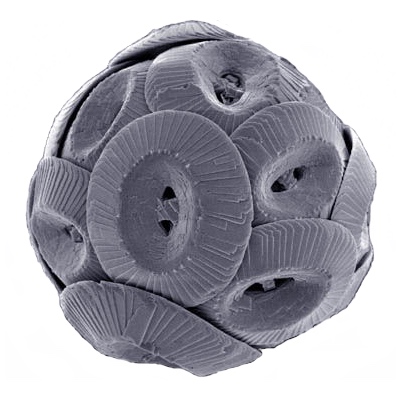
Figures \(\PageIndex{8}\) Above: coccolithophores
Coccolithus pelagicus is covered with a CaCO3 shell, a coccosphere. These are very small single-cell algae that form interlinked calcium carbonate circulate plates that cover the surface.
Figures \(\PageIndex{6-8}\): Some phytoplankton. Diatoms: https://commons.wikimedia.org/wiki/C...le:Diatom2.jpg; photosynthetic dinoflagellates: https://commons.wikimedia.org/wiki/F...lagellates.jpg; coccolithophores: https://commons.wikimedia.org/wiki/F..._pelagicus.jpg
Along the coast in summer, nutrient-rich upwelling can lead to the explosive growth of dinoflagellates, turning the water red-gold (often called a red tide). Some species in these blooms produce neurotoxins such as saxitoxin (an inhibitor of sodium channels), which can produce paralytic shellfish poisoning if shellfish from the bloom area are eaten, and brevetoxin (which stimulates voltage-gated sodium channels in nerve and muscle).
Ice cores from Antarctica and Greenland can extend to over 3.4 km (2.1 miles) in depth and yield direct information on CO2 and indirect temperature measurements. Until recently, continuous ice core records covered 130,000 years in Greenland and 800,000 years in Antarctica. Remarkably, a single continuous ice core 2,800 meters (1.74 miles) long that extends to the bedrock in Antarctica, dating back 1.2 million years, is now available. Analysis of this core might reveal the cause of the extension of the glacial cycle from 40,000 to 100,000 years, starting around 1 million years ago. Data spanning 2 million years is available from discontinuous cores. Concentrations of trapped CO2 as a function of time and the temperature of each layer in these cores can be determined. Figure \(\PageIndex{9}\) shows a section of an ice core from the West Antarctic Ice Sheet Divide (WAIS Divide).
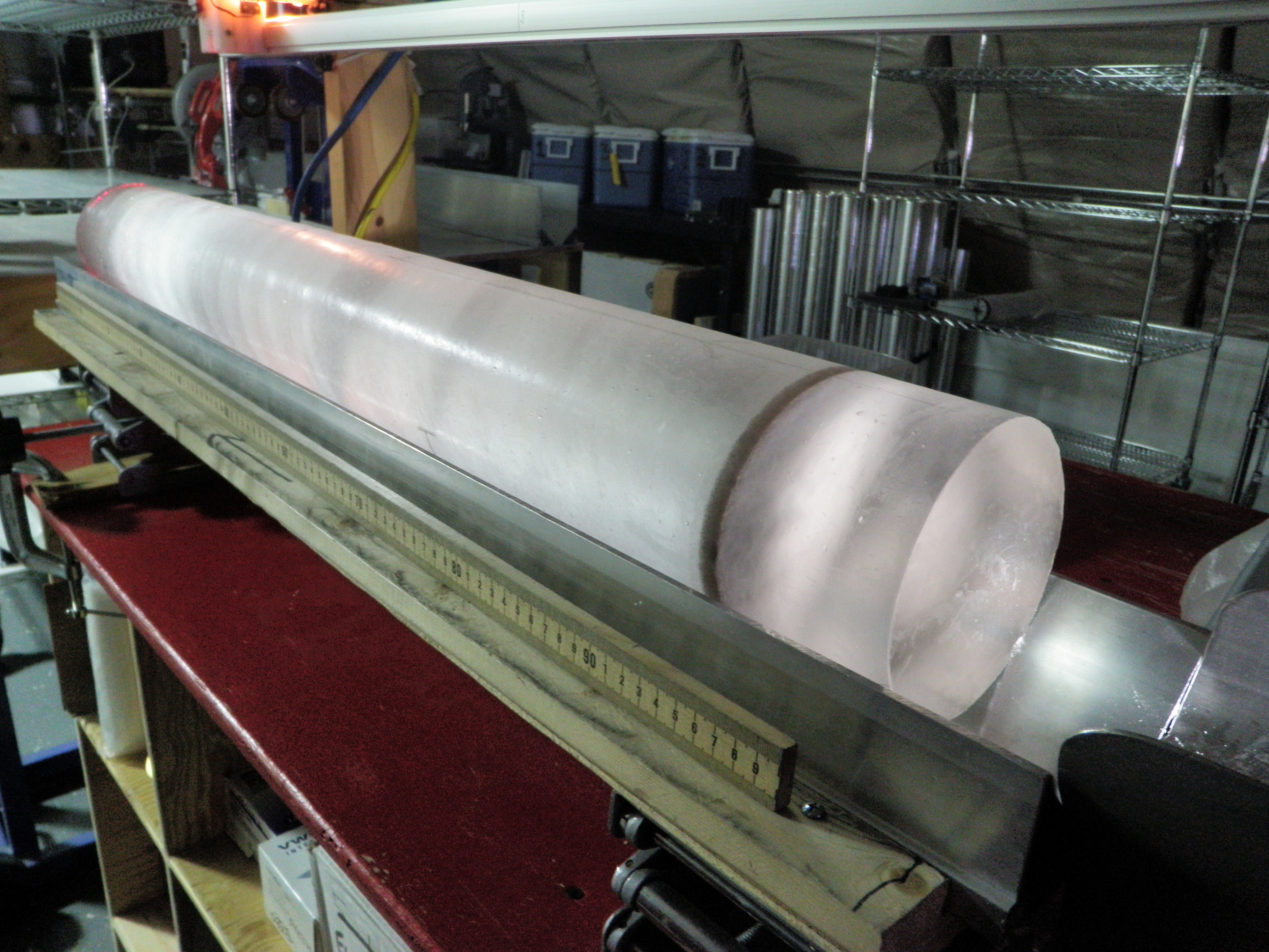
Figure \(\PageIndex{9}\): The dark band in this ice core from the West Antarctic Ice Sheet Divide (WAIS Divide) is a layer of volcanic ash that settled on the ice sheet approximately 21,000 years ago. Credit: Heidi Roop, NSFhttps://icecores.org/about-ice-cores
The remains of plankton shells described above are found in sea sediment cores. Analyses of shells, especially those of foraminifera, have provided climate data dating back tens of millions of years. For ice and ocean sediment cores, isotope analyses have been the key to obtaining CO2 and temperature data.
Isotope Analyses
To analyze ice and ocean sediment cores, three things are needed: the age of the layer, a direct or indirect measure of atmospheric CO2 at the time the layer was deposited, and an indirect measure of the temperature at the time of deposition. As shown in the figure above, ice core samples have rings, similar to trees, that can be used to count backward in time. The rings get harder to distinguish the further back you go. Figure 3 above shows a visible dark band deposited by volcanoes 21,000 years ago. Ultimately, isotopic analyses of H2O and CO2 in ice samples and of carbonates in minerals from deposited microfossils in ocean samples are critical in determining past CO2 and temperature values.
Most readers are familiar with 14C radiocarbon dating and 13C-NMR. Metabolic pathways have been elucidated using 2H (deuterium), 3H (tritium), 13C, and 14C to label specific atoms in substrates and follow their flow into products. These same isotopes have been used in kinetic experiments to determine enzyme reaction mechanisms. In this section, we will explore isotopes in some detail.
Use of unstable radioactive isotopes
14C radiocarbon dating is limited in climate analyses due to its short half-life (t1/2 = 5730 years). In contrast to most isotopes made in stellar nucleosynthesis or by the radioactive decay of a precursor radioactive element to an isotope of another element, 14C is made continually in the atmosphere when high-energy neutrons (n) from solar radiation react with atmospheric nitrogen (N). The neutron kicks out a proton to form 14C, as shown in the nuclear reaction below.
\[ n+{ }_7^{14} \mathrm{~N} \rightarrow{ }_6^{14} \mathrm{C}+p
\]
14C becomes oxidized to form 14CO2,which can enter the carbon cycle and the organic carbon pool through uptake by photosynthetic organisms and organisms that consume them. It can also form inorganic bicarbonate and carbonate ions, which could enter shells.
All living things take in 14C until their death, after which 14C decays through converting a neutron to a proton, a beta particle (electron), and an antineutrino, forming stable 14N. Hence, 14C in dead organisms or their remains decays with a t1/2 of 5730 years, in a process unaffected by temperature or pressure. 14C dating can be used on samples dating back about 55,000 years, a timespan representing 9.6 half-lives. Only 0.13% of the original 14C would be left. Data from this method provides the organism's age at death.
Carbon-14 dating assumes that the amount of carbon-14 in the environment is constant. However, the burning of fossil fuels and detonation of nuclear weapons have altered its amount (see box below). Changes in solar activity and the resulting changes in high-energy neutrons also affect the amount of carbon-14. Also, given the relatively short time frame of 14C dating, differences in CO2 based on its sequestration and circulation in the oceans are factors. Oceans cover 61% of the Northern Hemisphere compared to 81% of the Southern Hemisphere. Books on calibration factors can be used to control these effects. The calibrations are based on data from tree rings, lake and ocean sediments, corals, and stalagmites, which date back 55,000 years.
In the 1950s up to 1962, nuclear weapons were tested in the air, doubling the amount of 14C in the air. Organisms and the ocean have taken up this 14C spike. Also, since then, the amount of CO2 from burning fossil fuels has increased dramatically. This source does not contain 14C because it derives from fossils that have long since decayed. The effects canceled each other in 2021. Since 2021, more CO2 from fossil fuels has been added, so the net effect is now lower levels of 14C, equivalent to preindustrial time. It will continue to lessen until well after we stop using fossil fuels. By 2050, the levels might be equivalent to those in the Middle Ages. This, and the human-made halt to the next ice age glaciation cycle, are yet another warning about our effects on the entire biosphere.
The decay of other "unstable" radioactive isotopes is used for dating samples and determining the age of burial:
- 39Ar, an extremely rare isotope (t1/2 =269 yr), has been used to date ice cores from the Tibetan Plateau over the last 1,300 years.
- 40K (t1/2 = 1.25 billion yr) decays to 40Ar (stable), so their ratios can be used to determine how much time has passed since magma solidified into rock, based on diffusion rates of the resulting stable 40Ar.
- The 26Al/10Be ratio in buried samples is used in dating analyses. The two isotopes are rare and are produced in a fixed ratio (6.75/1) when formed in surface quartz by solar radiation (much as 14C is produced). When buried through geological processes, there is no further production of the isotope, but fortunately (for those who measure the age of burial), they decay with different half-lives (t1/2 = 717,000 yr for 26Al and t1/2 = 1.39 million yr for 10Be)
- The ratios of 21Ne/26Al and 21Ne/10Be can be used. 21Ne is a stable isotope, and these ratios are independent of the 26Al/10Be rate.
- Uranium isotopes are widely used to measure age on a long-term time scale. 238U (t1/2 =4.45 billion yr) is converted to 206Pb (stable) and 235U (t1/2 =704 million yr) to 207Pb (stable) by parallel decay routes, which allow for multiple types of dating measurement.
Use of stable isotopes
Most of the data and graphs of CO2 and temperature vs time (years ago) presented in Chapter 31.1 were determined using stable isotopes that do not decay. Much of the data is based on the ratio of the stable isotope pairs of oxygen (18O/16O) or carbon (13C/12C) in buried ice or ocean sediment cores. These isotopes have also been used to infer temperatures or temperature changes when targets were buried in ice cores or ocean sediments. Temperatures at the time of water deposition in ice layers are often inferred from 18O/16O ratios in the layers.
Ice core 18O/16O analyses
The oceans are vast and generally homogeneous reservoirs that can provide clues to long-term climate change. Short-term climate change would have limited effects on the oceans. The 18O/16O ratios in Greenland and Antarctic ice cores have enabled dating and temperature reconstruction over 800K years ago to even longer, since the ratio is determined by the 18O/16O in the liquid oceans at the time of ice formation.
The natural abundances of 18O (0.205 %) and 16O (99.757 %) give a ratio of the two isotopes of 0.0021, which is so small that the exact ratio is inconvenient for routine use. Rather, a comparison of the ratios in a target sample vs a universal reference, the δ18O value, is determined using a mass spectrometer. The δ18O value is calculated using the following equation:
\[ \delta^{18} O=\left[\frac{\left(\frac{18}{16} O\right)_{\text {sample }}}{\left(\frac{18}{16} \mathrm{O}\right)_{\text {reference }}}-1\right] * 1000
\]
Similar δ values are determined for D/H ratios (δ2H) and for 13C/12C (δ13C)
- The reference for δ18O calculations is the Standard Mean Ocean Water (SMOW or V-SNOW)
- The δ2D reference value is also based on SMOW or V-SNOW
- The standard for the analogous δ13C value is the Cretaceous Peedee Belemnite (an extinct order of squid-like cephalopods with an internal cone skeleton) sample from the Peedee Belemnite (PDB) formation in South Carolina, USA. This standard is no longer available, so an alternative, NBS 19, a carbonate material, is used in a new V-PDB (Vienna-PDB) scale.
| Element ratio | Ratio of natural abundance | Reference ratio |
|---|---|---|
| 18O/16O | 0.205/99.757 = 0.00205 | 0.0020052 (SMOW or V-SMOW) |
| 13C/12C | 1.1/98.9 =0.0111 | 0.011238 (PDB or V-PDB) |
| 2H/1H (D/H) | 0.0156/99.9844 = 0.000156 | 0.00015576 |
Note that the ratios of the standards, and likewise of the samples, are small. Also note that in the equation for δ18O, the bracketed term is multiplied by 1000.If multiplied by 100, the value for δ18O would be a percentage. Instead, it's multiplied by 1000 to convert it to per mill (per mil or ‰) or parts per thousand (just like percent is parts per 100). Hence 1‰ is 1 part per 1000 or 0.1%.
Equations can be just collections of letters with little intuitive meaning, or the user can deconstruct them to make intuitive sense. To help readers understand this equation, which most have likely never encountered, given its importance in climate studies, let's look at three sets of conditions. If ...
- 18O is enriched in the sample compared to the reference, then (18O/16O)sample/(18O/16O)reference is >1, so subtracting 1 makes the bracketed term +, along with δ18O;
- 18O in the sample is equal to that in the reference, then (18O/16O)sample/(18O/16O)reference =1, so the bracketed term = 0, and δ18O = 0;
- 18O in depleted in the sample compared to the reference, then (18O/16O)sample/(18O/16O)reference <1, so the bracketed term is -, along with δ18O.
A sample with a higher 18O/16O ratio (enriched in the heavier isotope) than the SMOW reference will have a positive (+) δ value. If the 18O/16O ratio of the substance is lower (depleted in the heavier isotope) than the SMOW reference, the δ value will be negative (-). The δvalues of SMOW (O and H isotopes) and PDB (C isotopes) are zero as they are compared to themselves.
Now let's examine ice and ocean δ18O values and see how delta values are used as proxies for temperature or changes in temperature at deposition.
The ice shields form from snow that forms from water evaporated from the oceans. Water can have multiple isotopic compositions, but based on the % abundances, the most likely ones are H216O and H218O. The lighter H216O evaporates more readily from the mid-latitudes of the oceans, and when it reaches the poles, condenses to form snow and eventually ice enriched in H216O. Urey showed that the vapor pressure of H218O is about 1% less than that of H216O between 46.35°C and 11.25°C.
In addition, the H218O that evaporates at lower latitudes is more likely to condense and be removed in rain, leaving the southern oceans enriched in H218O. This effect is quite significant: water, in the form of ice, in Greenland and Antarctica has about 5% less H218O than water at 20 0C from midlatitudes, making the δ18O of water a proxy for temperature but even better as a measure of ice volume and from that sea levels.
Now consider the Ice Ages, when oceans were enriched in H218O. During glacial melting of H216O-enriched ice, with meltwater flowing into the oceans, H218O would get diluted with H216O. At the same time, sea salinity would decrease because ice forms without ocean salts. These differences in H218O/H216O values in ice core samples are converted to δ18O values, which can be positive or negative, as shown in Figure \(\PageIndex{10}\).
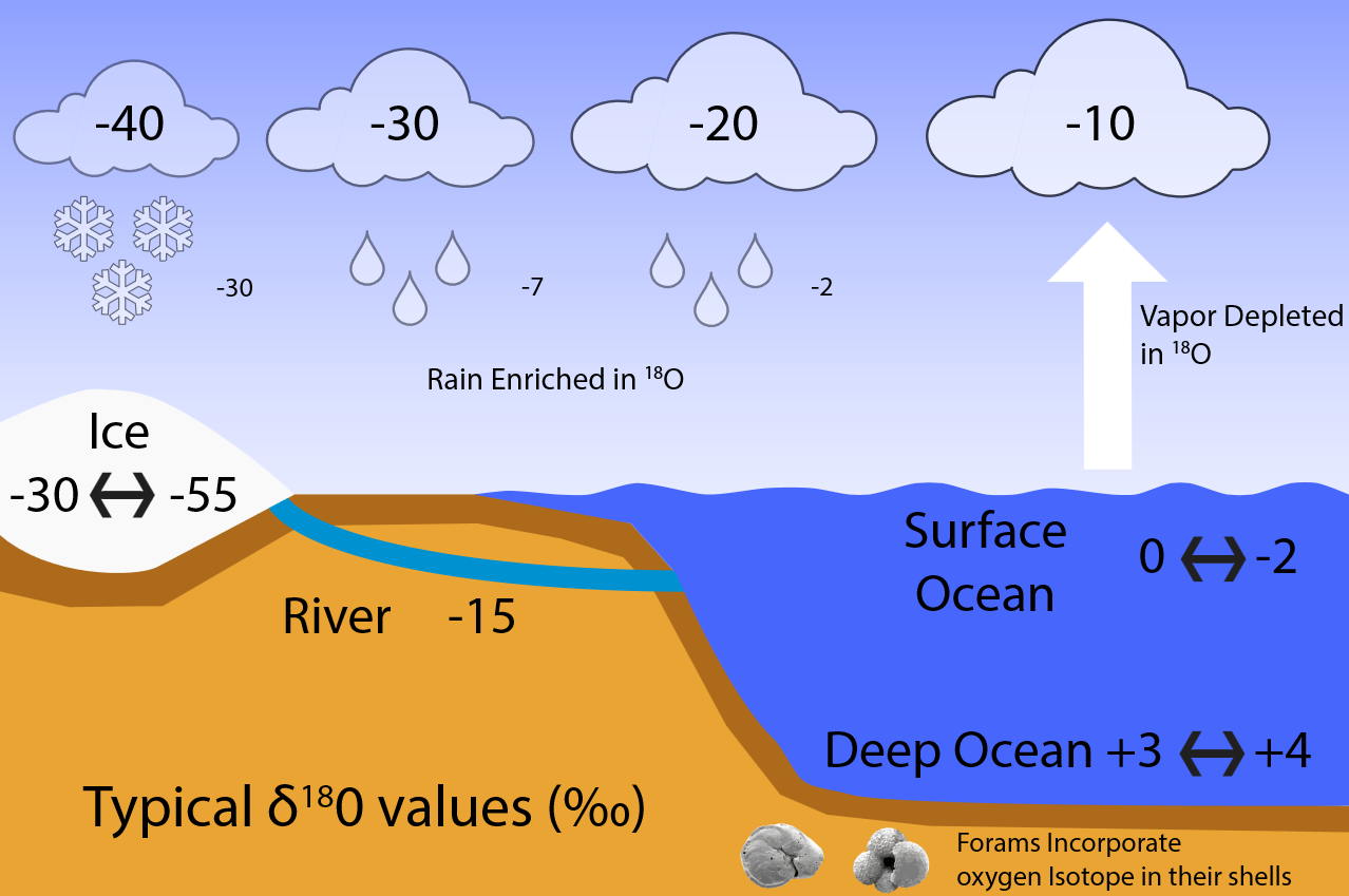
Figure \(\PageIndex{10}\): Typical δ18O values (in permil). Andreas Schmittner. https://eng.libretexts.org/Bookshelv...A_Paleoclimate
Surface ocean water has δ18O values of around zero. Due to fractionation during evaporation, less heavy isotopes are incorporated into the air, which leads to negative delta values of around -10 ‰ for the evaporated water vapor. Condensation prefers the heavy isotopes, as described above. In this example, the first precipitation thus has a δ18O value of about -2 ‰,(more positive than the first vapor). The remaining water vapor will be further depleted in 18O relative to 16O, and its δ18O value will become more negative (-20 ‰). Any subsequent precipitation event further depletes 18O. This process, known as Rayleigh distillation, results in very low δ18O values of less than -30 ‰ for snow falling onto ice sheets. Thus, ice has a very negative δ18O of between -30 and -55 ‰. Deep ocean values today are about +3 to +4 ‰. During the last glacial maximum, as more water was locked up in ice sheets, the remaining ocean water became heavier in δ18O by about 2 ‰. Foraminifera build their calcium carbonate (CaCO3) shells using the surrounding seawater. Thus, they incorporate the oxygen-isotopic composition of the water into their shells, which are then preserved in sediments and can be measured in the lab. Bralower and David Bice. https://www.e-education.psu.edu/earth103/node/5. Creative Commons Attribution-NonCommercial-ShareAlike 4.0 International License(link is external).
In summary, Greenland and Antarctic ice is enriched in 16O during cold conditions since H216O preferentially evaporates, condenses, and freezes into ice at the poles. In addition, as we will see below, deep-sea Foraminifera shells contain more 18O in shells since water is enriched with H218O in cold conditions, since less evaporates. Hence, δ18O becomes more positive.
The interactive graph below shows how Rayleigh Distillation drives changes in δ18O in polar ice as a function of temperature at the tropics and at different latitudes. Move the sliders to see the calculated δ18O values.
Ocean sediment core 18O/16O analyses
In the last section, we looked at δ18O values in ice core layers and their use as proxies for land and ocean temperatures and, more fundamentally, as indicators of ice volume, affecting sea levels and ocean salinity. It's amazing what we can surmise about past climate based on the fact that H216O evaporates more readily than H218O, and that H218O that did evaporate condenses at low and mid-latitudes more readily than H216O. These two factors lead to the enrichment of H216O in polar ice and H218O in low and mid-latitude ocean water. Remember that evaporation and condensation are physical reactions involving a state change.
Yet ice cores extend only so far back in geological time. To go back further, scientists analyze shells buried in ocean sediments. More specifically, they analyze the 18O/16O isotopic ratio in calcium carbonate (calcite, CaCO3) from the buried shells of organisms such as foraminifera. (Calcite is a stable anhydrous form of CaCO3, but it can form different calcite phases under high pressure.) Now, we are dealing with a new atom, C, in the carbonates. Hence, the interpretation of δ18O in buried carbonate is influenced by more factors than in solid or liquid water. It must include these factors
- the chemical reactions of inorganic carbonate formation (precipitation) and dissolution (compared to the physical reactions of water evaporation and condensation)
- the biological formation of CaCO3 in shells
- an understanding of the carbon cycle
- the temperature at which the CaCO3 was deposited
- the salinity at deposition, as the formation of CaCO3 from its ions, and the overall ionic strength of the medium in which CaCO3 formed, would influence the thermodynamics and kinetics of how the separate ions approach each other to form the solid
- equilibrium and kinetic controls of the precipitation reactions.
We will see below that Foraminifera shells in ocean core samples contain more 18O in cold conditions because H218O iis enriched in those conditions. Hence, δ18O becomes more positive.
To truly understand biochemistry, we must include both biological and chemical aspects. Biochemistry requires synthesizing knowledge from many disciplines, including introductory chemistry (where precipitation reactions were likely first covered) and analytical chemistry (which delves more deeply into them). Hence, we don't apologize for bringing back your previous knowledge of precipitation reactions. At the same time, our description of the use of δ18O values in buried ocean sediments is very simplified.
We must consider two reactions to understand δ18O values in calcite Foraminifera shells. The first describes how 18O gets into CO32- in the first place. The second describes the seemingly simple reactions to form CaCO3 from its ions.
Enrichment of CaCO3 with 18O
The reaction below best describes the incorporation or fractionation of 18O from H218O into calcite shells.
Fractionation Reaction: (1/3) CaC16O3 + H218O → (1/3) CaC18O3+ H216O
In this reaction, the most abundant source of 18O is H218O. Figure \(\PageIndex{11}\) shows a simplified reaction mechanism.

Figure \(\PageIndex{11}\): Incorporation of 18O into carbonate from H218O
More broadly, there would be an exchange of isotopes in the entire dissolved inorganic pool (DIC) = CO2(aq) + H2CO3 + HCO3− (bicarbonate) + CO32− (carbonate) with H2O.
Formation of CaCO3
Two reactions in general describe calcite formation and its growth:
\[ \mathrm{Ca}^{2+}(\mathrm{aq})+\mathrm{CO}_3^{2-}(\mathrm{aq}) \leftrightarrow \mathrm{CaCO}_3
\]
and
\[ \mathrm{Ca}^{2+}(\mathrm{aq})+\mathrm{HCO}_3^{-}(\mathrm{aq}) \leftrightarrow \mathrm{CaCO}_3+\mathrm{H}^{+}
\]
These show that the uptake of 18O into CaCO3 should also take HCO3- into account
In an environmentally controlled laboratory setting, reaction 3 above can be considered to be at equilibrium and defined by a Ksp value, as you learned in introductory chemistry courses, in which reaction is written as the dissociation of the two ions from the solid.
Chapter 4.12 discussed the relationships between Keq, ΔG0, ΔH0, DS0, and temperature. There is an inverse relationship between Keq and temperature.
\begin{equation}
\begin{gathered}
\Delta \mathrm{G}^{0}=\Delta \mathrm{H}^{0}-\mathrm{T} \Delta \mathrm{S}^{0}=-\mathrm{RTln} \mathrm{K}_{\mathrm{eq}} \\
\ln \mathrm{K}_{\mathrm{eq}}=-\frac{\Delta \mathrm{H}^{0}-\mathrm{T} \Delta \mathrm{S}^{0}}{\mathrm{RT}} \\
\ln \mathrm{K}_{\mathrm{eq}}=-\frac{\Delta \mathrm{H}^{0}}{\mathrm{RT}}+\frac{\Delta \mathrm{S}^{0}}{\mathrm{R}}
\end{gathered}
\end{equation}
Assuming that the formation of CaCO3 is in equilibrium, you would expect that CaCO3 would be enriched in 18O and have a +δ18O value. Let's see why.
Urey showed that, under equilibrium conditions, calcite is slightly enriched in C18O32- probably because the heavier carbonate has a lower vibrational energy, which favors its stability and the formation of the solid. In addition, the incorporation of 18O is even more pronounced in colder water, which, as we have seen, has a +δ18O value (given the greater propensity of H216O to evaporate).
Hence, in cold periods with large ice shields, δ18O values from shells of foraminifera living in the illuminated upper ocean (planktic foraminifera, which engage in photosynthesis) and deep-sea benthic foraminifera are more positive. When ice shield melts, the δ18O values of water become more negative, and so do the values of δ18O values of the foraminifera.
- As planktic forams live in the upper ocean (0–200 m), their δ18O values are determined by surface ocean temperature and the seawater δ18O. Planktic foraminifera δ18O values are proxies for local temperatures because they are in a more dynamic, less-mixed environment and are more affected by evaporation and precipitation.
- In contrast, benthic forams live on the sea floor at great depth, where the ocean temperature is relatively constant (~1–4°C). The δ18O values of their carbonate shells serve as proxies for global ice volume. As an example, when ice shields are large in periods of glaciation, the δ18O of the whole ocean increases, due to sequestration of more H216O in ice. At the last glacial maximum, sea levels were about 120–130 meters lower than today (about 3% of the total ocean volume). Benthic foraminifera give a global temperature estimate as deep waters are more homogeneous.
Yet the formation of CaCO3 in shells in many cases is not in equilibrium and is in part determined by the concentration of the reactants, the rate of diffusion of ions into and out of the growing calcite shell, which would also depend on salinity (affecting electrostatic attractions of the ions to the growing crystal), the pH (which affects the ratio of CO32− and HCO3−) and biological effects (from the mechanism by which shells are formed which at some point may involve HCO3− transporters). It also depends on the transfer of carbonate within the dissolved inorganic carbon pool (DIC). The reaction is in equilibrium in some species of foraminifera but not others.
The term fractionation is often used in the isotope and climate literature (as we saw with Ralyleigh fractionation of H216O in polar ice). Using water as an example, fractionation describes the ratio of heavy to light O isotopes as they partition between the liquid, solid, and gas phases. The fractionation factor determines the δ18O value of water. Likewise, a fractionation process determines the partitioning of 18O from water into CO32- and CaCO3during calcite precipitation. The fractionation factor α is the ratio of the isotopes' changes in a physical (e.g., a phase transition) or chemical process. It is the factor by which the abundance ratio of two isotopes will change during a chemical reaction or a physical process.
In controlled studies of calcite (CaCO3) formation from HCO3−, the CaCO3 exhibits different oxygen isotope concentrations depending on the initial concentrations of reactants. The size of a shell can also affect the δ18O of additionally deposited CaCO3. These ideas support the notion that isotopic fractionation in CaCO3 occurs through both equilibrium and kinetic processes.
Hence, δ18O of shells depends on two environmental signals:
- temperature at the time of shell formation and
- seawater δ18O (which depends of global ice volume).
This makes the interpretation of δ18O values in ocean cores more challenging. Theoretical "paleotemperature" equations have been developed to relate temperature T to δ18O in calcite under equilibrium conditions.
One recent calibration equation for the formation of calcite from HCO3- (obtained by bubbling the reaction mixture with N2 at various temperatures) was derived by Kim and O'Neil in 1997. The equation was derived from carefully controlled laboratory studies that apply under equilibrium conditions and is shown below. The Kim and O’Neil equation shows the relationship between the fractionation factor alpha (α) of 180/160 between inorganically precipitated CaCO3 (calcite) and H2O as a function of temperature is shown below.
\[ 1000 \ln \alpha\left(\text { Calcite- } \mathrm{H}_2 \mathrm{O}\right)=18.03\left(10^3 T^{-1}\right)-32.42
\]
Alpha is the fractionation factor, and T is in Kelvin. Note: An update of this equation to conform to IUPAC conventions gives 103 ln α = 18.04 x 1000 / T - 32.18)
The oxygen isotope fractionation factor alpha between two substances, A and B, is defined as
\[ \alpha=\left({ }^{18} \mathrm{O} /{ }^{16} \mathrm{O}\right)_{\mathrm{A}} /\left({ }^{18} \mathrm{O} /{ }^{16} \mathrm{O}\right)_{\mathrm{B}}
\]
The left-hand side of the equation (1000xlnα) is used for convenience, and its relationship to δ18O values (which are expressed per %o) is analogous to the use of pKa = -log[KA] instead of KA.
An alternative form of the Kim and O'Neil equation is expressed in quadratic form.
\[ T\left({ }^{\circ} \mathrm{C}\right)=16.1-4.64 \cdot\left(\delta^{18} \mathrm{O}_{\mathrm{calcite}}-\delta^{18} \mathrm{O}_{\mathrm{water}}\right)+0.09 \cdot\left(\delta^{18} \mathrm{O}_{\mathrm{calcite}}-\delta^{18} \mathrm{O}_{\mathrm{water}}\right)^2
\]
A controlled equilibrium study using cultured foraminifera B. marginata of different sizes at different temperatures yielded an experimental equation to compare several theoretical equations. Figure \(\PageIndex{12}\) shows graphs of the empirically determined equation (non-red lines) vs the theoretical Kim and O'Neil equation (red line).

Figure \(\PageIndex{12}\): Comparison of experimental calibration equation with the theoretical equation for equilibrium calcite of Kim and O’Neil (1997). Barras, Christine & Duplessy, J.-C & Geslin, Emmanuelle & Michel, Elisabeth & Jorissen, Frans. (2010). Calibration of δ18O of cultured benthic foraminiferal calcite as a function of temperature. Biogeosciences. 7. 1349-1356. 10.5194/bg-7-1349-2010. CC Attribution 3.0 License
The brown, blue, and green lines represent the calibration equations for cultured B. marginata from the < 150, 150–200, and 200–250 μm size fractions, respectively. The red line represents the quadratic equation derived from the Kim and O’Neil (1997) relationship.
A quick inspection of the empirical equation for different sizes of B. marginata shows the same relationships between T and δ18O values as shown in Table \(\PageIndex{5}\) below. (The f and w in the equation represents forams (calcite) and water, respectively)

Table \(\PageIndex{5}\): Best fit linear plot of temperature T vs. (δ18Of - δ18Ow) for foraminifera B. marginata vs. size, where the subscript f is foraminifera, and w is water.
We take this "deep dive" into how oxygen isotopes in ice and deposited shells in ocean core samples give you a basic understanding of how creative and rigorous scientists have been in reconstructing past climates. To reiterate, during a glacial period, foraminifera shells become enriched in 18O for two reasons:
- cold water fractionates more strongly, giving shells more enriched in 18O
- ¹⁶O is preferentially locked in ice sheets, making sedimented shells enriched in 18O
In a simplified form, this can be expressed as:
\begin{equation}
\Delta \delta^{18} \mathrm{O}_{\text {foram }}=\Delta \delta^{18} \mathrm{O}_{\text {temperature }}+\Delta \delta^{18} \mathrm{O}_{\text {ice volume }}
\end{equation}
These effects are separated through a combined analysis of deep- and surface-water samples.
The interactive calculator below provides insights into the controls on Foram Shell δ18O. Use the sliders to calculate the foraminifera calcification temperature and explore how temperature and ice-volume effects contribute to the measured δ18O signal. The calculator was produced using Claude AI.
p>
Click for more details
- Answer
-
The Mg/Ca ratio in foram shells is a temperature-only proxy — magnesium substitutes for calcium in the calcite lattice more readily at higher temperatures. There is one big difference: the Mg/Ca ratio is not sensitive to seawater δ¹⁸O or ice volume, so it gives you temperature independently of the isotope signal.
If you measure both Mg/Ca and δ¹⁸O on the same foram shells, you can use Mg/Ca to determine the calcification temperature, then use that to calculate what δ¹⁸O the shell should have from temperature alone. The difference arises from ocean water δ¹⁸O, which reflects global ice volume.
We take this opportunity to reshow the graph that reconstructs changes in planetary temperatures over the last 66+ million years (Figure \(\PageIndex{13}\)). Data between 66 MYA and 100,000 years ago (note the change in scale on the x-axis to fit a large time range in a single graph) were obtained, partly from δ18O values in deep-sea sediments. In contrast, data from around 100,000 YA to the advent of modern temperature recordings were mostly obtained from δ18O measurements of ice core samples from Antarctica and Greenland. Of course, other temperature proxies, as described above, were also important.

Figure \(\PageIndex{13}\): https://commons.wikimedia.org/wiki/F...alaeotemps.png. (Excel available). Creative Commons Attribution-Share Alike 3.0 Unported
These detailed but hopefully understandable explanations of the relationship of temperature with δ18O in foraminifera shells from ocean sediment cores were presented for reasons expressed at the beginning of Chapter 31.2:
- Isotopes and their effects are critical to understanding the structure and activity of biological systems and to climate science.
- Isotope partitioning into water and biomolecules involves both equilibrium and nonequilibrium reactions and processes, similar to linked biochemical reactions and pathways.
- The study and application of isotope effects can integrate and expand learning from previous science courses.
Astute readers will notice that we concentrated on δ18O values (in water and carbonates) and barely mentioned δ13C values for carbonate precipitations. We will discuss that in the next chapter as we consider the carbon cycle.
Summary
This chapter delves into the sophisticated methods used to reconstruct past atmospheric CO₂ levels and global temperatures over millions of years using isotope analyses. It highlights how scientists extract and interpret data from ice cores and ocean sediment cores—key records that have preserved information in the form of isotope ratios of oxygen (δ¹⁸O) and carbon (δ¹³C). The chapter emphasizes the following points:
-
Isotope Fundamentals and Their Significance:
The study begins by outlining why isotope effects are crucial not only for understanding biochemical structures and reactions but also for decoding Earth’s climate history. The partitioning of isotopes into water and biomolecules involves both equilibrium and non-equilibrium processes that mirror many biochemical pathways. -
Proxies for Past Climate Reconstruction:
Since direct measurements of temperature and CO₂ are available only from recent centuries, scientists rely on “proxies” such as tree rings, coral growth bands, and the shells of marine organisms (e.g., foraminifera, diatoms). These proxies, calibrated against modern observations, allow researchers to infer past temperature variations and atmospheric CO₂ levels extending back millions to billions of years. -
Isotope Analyses in Ice and Sediment Cores:
The chapter explains how isotopic ratios—especially ¹⁸O/¹⁶O—in ice cores from Antarctica and Greenland serve as indicators of past temperature changes and ice volumes, while similar analyses of carbonate shells in marine sediments provide complementary data on ocean temperatures and global climate trends. -
Chemical Reactions and Fractionation Processes:
Detailed discussions focus on how isotopic fractionation occurs during the evaporation and condensation of water and the precipitation of calcium carbonate (CaCO₃) in foraminifera shells. The theoretical framework, including the Kim and O’Neil calibration equations, illustrates how temperature influences isotope partitioning and thus the δ¹⁸O values measured in climate proxies. -
Interdisciplinary Integration:
Finally, the chapter underscores the importance of integrating knowledge from chemistry, biology, and geology. By linking the study of isotope effects in biochemical systems to their application in climate science, students gain a comprehensive understanding of how ancient climate records are constructed, validated, and used to inform models of future climate change.
Overall, this chapter provides junior and senior biochemistry majors with both the theoretical background and practical applications of isotope analysis in reconstructing Earth’s climatic history, demonstrating how rigorous scientific methods underpin our understanding of global climate dynamics.