2: Back to the Present and Future of Climate Change

Back to the Recent Past and Present

Let's return to more recent human history and the anthropogenic forcing of our climate. Figure \(\PageIndex{14}\) shows an interactive graph of atmospheric CO₂ over more recent times. Zoom into the steep rise in CO₂ that started around 1760 with the Industrial Revolution.

Figure \(\PageIndex{15}\): Interactive graph of atmospheric CO₂ vs time over the last 1000 years. Historical CO₂ record from the Law Dome DE08, DE08-2, and DSS ice cores. Credits: D.M. Etheridge, L.P. Steele, R.L. Langenfelds, R.J. Francey and the Division of Atmospheric Research, CSIRO, Aspendale, Victoria, Australia. 2 Degrees Institute. https://www.2degreesinstitute.org/. Also, https://www.co2levels.org/

Orbital mechanics cannot explain the planet's warming in the brief (in geological terms) times since the Industrial Revolution. Neither can volcanic activity, changes in solar activity, changes in land use (for example, deforestation that slows down photosynthesis and CO₂ removal from the atmosphere), or even aerosols released on burning fossil fuels (which would decrease global temperature due to increased reflection of sunlight). Click on Figure \(\PageIndex{15}\) to see an animated explanation of which factors best explain the global temperature increase since 1880. The results are clear: It's us!

Figure \(\PageIndex{15}\): Factors contributing to global warming based on NASA data and NASA's Goddard Institute for Space Studies (GISS) climate models.

Unfortunately, other greenhouse gases have also risen since 1975, as shown in Figure \(\PageIndex{16}\).

Figure \(\PageIndex{16}\): Rise in greenhouse gases since 1975. https://www.co2.Earth/annual-ghg-index-aggi

Take special note of the zig-zag nature of the CO₂ curve. The curve dips a bit in the summer when plants in the Northern Hemisphere actively remove CO₂. Increasing methane now accounts for up to 20% of the warming observed. Figure \(\PageIndex{17}\) shows as an interactive graph of a very worrisome rise of atmospheric methane with time.

Figure \(\PageIndex{17}\): Interactive graph of atmospheric CH₄ vs time over the last 1000 years. 2 Degrees Institute. https://www.2degreesinstitute.org/

Present-day warming is unequivocally caused by humans burning fossil fuels.

Past Climate Anomalies

Several dramatic but short-lived (in geological time) climate changes have punctuated recorded human history. Let's look at two, mostly to equip you to address climate skeptics. They also show the sensitivity of our climate to subtle changes.

The Little Ice Ages 

Actual and proxy temperature records show a mild period in Europe from around 950-1100, followed by colder weather, especially from 1450 to 1850. The latter period is called the "Little Ice Ages," although no significant expansion of the North Hemisphere ice shield occurred. It was especially cold worldwide in 1816 when much of the world experienced a "year without summer." The effect in 1816 had a clear cause: the explosion of the volcano Mount Tambora in Indonesia on April 10, 1815.

In addition to this identifiable influence in 1816, a cool period was reported for the northern hemisphere from about 1800 to 1820, starting earlier than the Tambora eruption. Also, a low period of the sun's irradiance, the Dalton Minimum, occurs from 1790-1860. Proxies for solar activity in the 1600s also show small solar irradiance drops, as we will discuss below. The dip in global average temperatures following the Medieval warm period is shown in Figure \(\PageIndex{18}\).

Figure \(\PageIndex{18}\): Dip in global average temperatures following the Medieval warm period, By RCraig09 - Own work, CC BY-SA 4.0, https://commons.wikimedia.org/w/inde...curid=87832845

Modern climate changes have been captured in literature and art. One example is a painting showing "Ice Fairs" on the Thames in London, shown in Figure \(\PageIndex{19}\).

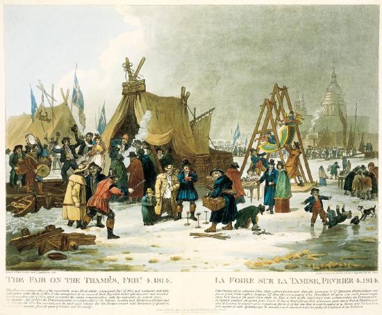
Figure \(\PageIndex{19}\):https://commons.wikimedia.org/wiki/F...enell.jpgdfdfd

Many factors probably contributed to the Little Ice Ages, including a drop in solar irradiance. A newer explanation has also been proposed. Marine records show that the water near Greenland and the Nordic seas was warmer, caused by a strengthening of the Atlantic Meridional Overturning Circulation (AMOC). This would have caused the loss of Arctic ice in the late 1300s and 1400s, cooling the water and diluting its salinity since ice, when it crystallized with a tetrahedral hydrogen-bonded coordination of water, excludes salt. This would have collapsed the AMOC and its heat transfer to the northern waters, leading to rapid and prolonged cooling. An analogous strengthening of the AMOC was observed between 1960 and 1980, which was attributed to a long-duration high-pressure system over Greenland. A similar event might have occurred to kick-start the Little Ice Ages. Tree rings show evidence of higher solar irradiance before the Little Ice Ages, which may be associated with the initial strengthening of the AMOC.

The Little Ice Ages also affected China and may have contributed to crop failure in 1644, when the Ming Dynasty fell. An Arctic hurricane in 1588 helped destroy the Spanish Armada. The Great Fire in London in 1666 was preceded by a very dry summer that followed an exceptionally cold winter. Food production was severely disrupted, which might have led to significant social change in Europe and elsewhere as the Plague shattered societal and cultural norms.

The explosion of Mount Tambora in present-day Indonesia in 1816 greatly exacerbated the effects of cooling. The ash and SO₂ aerosols block solar irradiance. Droughts, floods, cholera epidemics, famine, and migration from Europe to the US and East to West partly arose from this event.  

One of the worst times to be alive: 536

Historians report that in 536 AD, parts of Europe, the Middle East, and Asia experienced 24 hours of darkness for up to 18 months.  Summer temperatures plummeted. Famines occurred for a few years after. It snowed in China in the summer. The worst effects were in the Northern Hemisphere, but they were worldwide. It was probably the most pronounced cooling in the last 2000 years. To make matters worse, a pandemic erupted around 541, spreading from southern Asia to northern Europe. It had a huge effect on the Byzantine Empire and has been called the Justinian (bubonic) Plague after the Byzantine emperor. Crop failures, an expansion of trade, and an influx of rodents derived from the cold temperatures could have led to and exacerbated the plague.

This second and severe example of cooling was shorter-lived in a geological time frame. Temperatures fell in the summer about 1.5-2.5⁰C. A "smoking gun" has been linked to this cooling, a volcanic explosion in Iceland. In addition, another eruption occurred in 540, which dropped the temperature another 1.5-2.5⁰C, and in 547. The combined effects of climate change and the plague led to a significant economic fall in Europe. Signs of airborne lead in the ice in 640, arising from silver mining, suggest a recovery of economic growth. You should ask yourself how the modern world copes with such an occurrence. 

Solar Activity and Climate Change

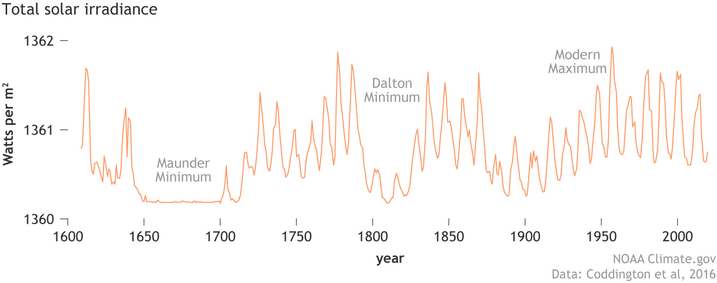
We have discussed how the orbital forcing of the climate kick-started each of the recurring ice ages in the Pleistocene. Some effects of the change in solar activity independent of the sun's orbit have been noted above. Specifically, we have shown that it cannot account for present warming. We present a series of graphs from the NOAA (National Oceanic and Atmospheric Administration) in the collective Figure \(\PageIndex{20}\) below to show the actual change in solar activity over recent times. Comments are shown at the bottom of each graph.

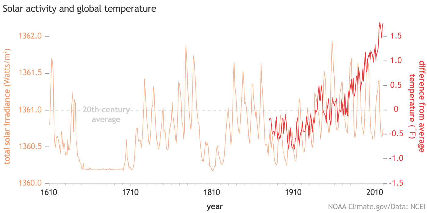
(Above) The maximal % spread from the lowest to the highest is very small. Such a small change shouldn't have such dramatic effects on climate unless sustained, as it was from around 1630-1700. Hence, this decline in solar activity probably played a part in the Little Ice Ages. The regular rise and fall (spikes) are associated with the 11-year sunspot cycle activity. Note that the rise in average temperature since 1910 (shown in red) cannot be accounted for by change in solar activity

The above graph shows that the irradiance decreased by about 0.06% (although other values have been reported as high as 0.22%) during the Maunder Minimum, which occurred in the Little Ice Ages. The average decrease in terrestrial temperatures was 1.0-2 ⁰C.

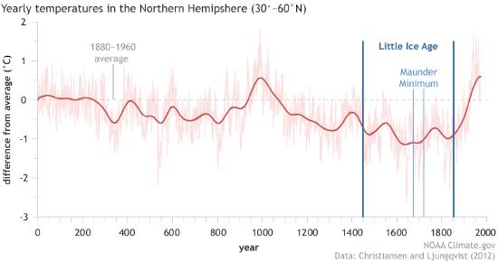
The graph above shows yearly average temperatures in the Northern Hemisphere. The dark red line shows the average change. Note that the averages are lower in the Little Ice Age with the lowest values and lowest spike temperatures close to and in the Maunder Minimum.

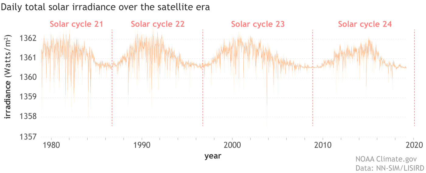
(Above) The 11-year repeat of sunspot activity and resulting solar irradiance is seen in the graphs. In 2020, a low in activity occurred, yet 2020 was the second warmest year on record since 1880.

This graph does not show the effects of climate forcing due to orbital changes. Rather, it shows that solar activity did not change significantly for the 10,000 years before 0 CE.

Figures \(\PageIndex{20}\): Solar activity changes in recent geologic time.

This would be true if not for the massive amount of CO₂, approximately 1.5 trillion tons, injected into the atmosphere since the Industrial Revolution from using fossil fuels. Not all of that is still in the atmosphere, but enough to raise CO₂ to levels not seen for 3 million years. Based on the relationship between CO₂ and temperature across the ice ages, science can predict when conditions might exist to initiate and propagate the next ice age. The data arising from these models, illustrated in Figure \(\PageIndex{21}\), show how much incoming solar radiation (insolation) must arrive at the Earth (watts/m²) to trigger the next ice age.

Figure \(\PageIndex{21}\): Incoming solar radiation required to trigger the next ice age.

As shown in the left side of the figure, if CO₂ were 280 ppm (typical of peaks in past interglacial periods), it would take repetitive insolation drops below the threshold of about 455 watts/m² (red line) to start glaciation. As of November 2022, we are at 415 ppm and rising. If it rises to 450 ppm, as it assuredly will in the absence of carbon capture, it would require much less insolation since the greenhouse effect of the higher CO₂ would warm the atmosphere The right graph shows there is little chance of another ice age in the absence of large and sustained volcanic activity or asteroid impact that would lead to blocking of solar radiation.

Summary of Climate Change Causes and Effects Since 900 AC

Figure \(\PageIndex{22}\) summarizes possible contributions to temperature change over the last 1000 years. Note again that our present warming can only be attributed to greenhouse gases (GHG). One panel shows changes in land use. This has caused a temperature drop since 1800. That effect is caused by deforestation and other land cover changes, which leads to more reflection of incident solar radiation back into space. This effect is increased in the winter if the changed land is snow-covered. Deforestation would also decrease CO₂ capture (photosynthesis) by plants, raising the temperature. That component has been added to the GHG panel. 

Figure \(\PageIndex{22}\): Simulated northern hemisphere temperature changes, smoothed with an 11-year running mean, relative to AD 950–1250. Owens et al. J. Space Weather Space Clim. 2017, 7, https://doi.org/10.1051/swsc/2017034. Creative Commons Attribution License (http://creativecommons.org/licenses/by/4.0).

The black line in the top panel shows the observed instrumental northern hemisphere temperature variations with their associated uncertainties (Morice et al., 2012), which match the simulations well. The bottom panel shows a simulation with no changes to the radiative forcings. This quantifies the magnitude of natural internal variability in the simulations without changes in forcings. Note periodic but short-term dips in temperature due to volcanic activity. Warming since the Industrial Revolution is due to emissions from the use of fossil fuels. 

Climate Justice: The Emitters and the Affected

We present a series of graphs in Figure \(\PageIndex{24}\) below, taken from CO₂ Emissions - Our World in Data, to show which countries have emitted the most CO₂ in the past and now. In a just world, those countries that have emitted the most should move swiftly and forcefully not only to decrease emissions but to aid other countries' transitions to clean fuels and to help them with climate change mitigation and adaptation. We don't wish to demonize the fossil fuel industry and those who work in it. The use of fossil fuels, which are high energy, high density, and cheap fuel (because of historically massive subsidies) has lifted millions if not billions out of poverty over time. We had no alternative to fossil fuels until recently. Most did not realize how significantly fossil fuel use would affect our present and future climate, human health, and the entire biosphere. (Yet there is evidence that.) We can't just stop the use of fossil fuels without inflicting great economic pain on those who can least afford it. To help those currently suffering and who will suffer most in the future and help ourselves, our children, and our grandchildren, we must move away from using fossil fuels as soon as possible.

Above: The dip in total world emissions in 2020 was due to the COVID-19 pandemic. Unfortunately, the rise has resumed. China is now the biggest net emitter, but the US and EU emissions are dropping. India is on the rise, and if it follows a similar economic path as China, which it needs to lift many out of poverty, it will come with a huge cost in CO₂ emission unless it can jumpstart their conversion to clean fuels. The world needs to help.

Above: Although China is the largest net emitter, the US and Australia are the biggest emitters per person, although that is dropping.

The US still leads the world in total CO₂ emitted since the Industrial Revolution. We also have the greatest GDP. Pakistan suffered tragical flooding, exacerbated by climate change, in 2022. Up to a 1/3 of the country was under water. In a just world, the biggest emitters would aid the rest of the world.

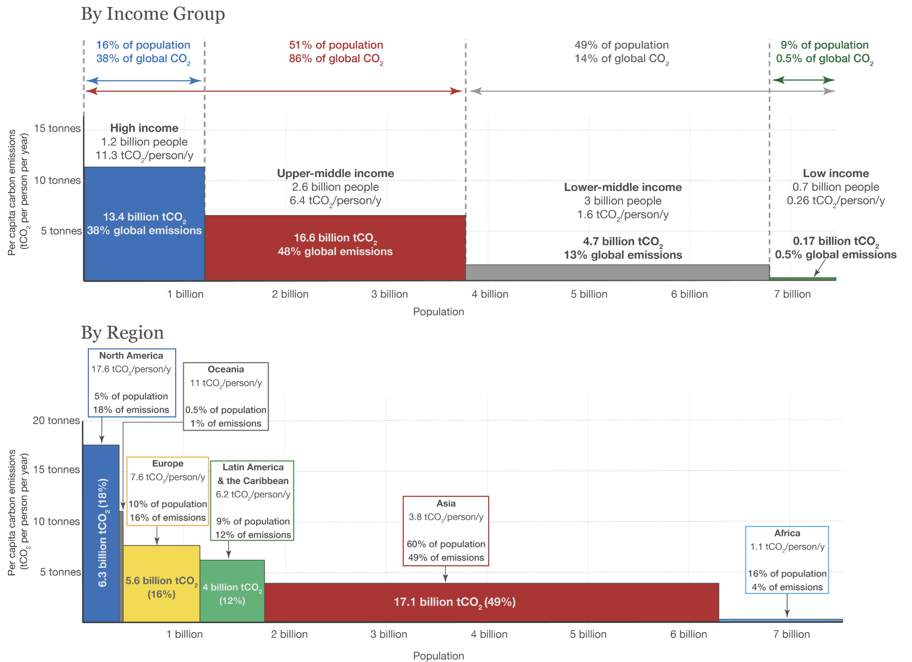
Above: Inequality is evident in this graph as the wealthiest people (high and upper-middle income) collectively contribute 86% of CO₂ emissions

Figure \(\PageIndex{24}\): CO₂ emissions by country and income since the industrial revolution. Our World in Data.  Creative Commons BY license. 

Future Projections

We know the science and the consequences if we choose not to act or act in ways insufficient to meet the challenges of climate change. It is one of the most difficult challenges we have faced as a species. It requires sacrifice and united action for the common good. The benefits of our choice are mostly in the future and for future generations. 

The Intergovernmental Panel on Climate Change (IPCC), composed of leading climate scientists and experts, has defined several different Relative Concentration Pathways (RCPs) leading to different emissions and climate futures. Where we end up depends on economic, social, and political choices. The IPCC initially designated four pathways, RCP 2.6, 4.5, 6, and 8.5, with higher numbers associated with higher temperatures and CO₂ levels. Each assumes a starting value and estimated emissions (which depend on technology, politics, economics, etc). RCP 8.5 assumes extra radiative forces (heat energy/(m²s)) by 2100 equal to 8.5 J/(s m²) or 8.5 watts/m². This worst-case scenario assumes business as usual with no interventions to reduce our emissions, a totally unlikely scenario given present actions (including the rapid rise of clean energy). The RCP 2.6 scenario assumes that the peak radiative forcing would be 3 watts/m^2, declining through strong governmental and economic actions to 2.5 by 2030-2040. Table \(\PageIndex{1}\) below shows the four RCP scenarios with projected ending CO₂ equivalents (which include other greenhouse gases) and temperature increases.

Translating the projected CO₂ equivalents in the atmosphere into associated temperature increases requires a high-quality value for climate sensitivity (rise in temperate/rise in CO₂). Figure \(\PageIndex{25}\) shows the likely temperature increase for the four scenarios.

The scenarios in Figure 25 are labeled SSP#-## with the second number ## representing the RCP number. The IPCC 6th report issued in 2021 changed from using RCP scenarios to Shared Socioeconomic Pathways (SSPs) scenarios based on possible social and economic developments that would pose different challenges to reduce future temperature increases and hence different strategies for mitigation and adaptation. The SSP scenarios are consistent with the RCP scenarios but use a more enhanced socio-economic and political framework for their construction. The mitigation strategies are based on the RCP forcing levels. The SSP scenarios are described below. They start with SSP1, which leads to a world that has adapted well and moved away from fossil fuels, to SSP5, which assumes a continued and high reliance on fossil fuels. 

SSP1:  Sustainability – Taking the Green Road (Low challenges to mitigation and adaptation)
The world is gradually but pervasively shifting toward a more sustainable path, emphasizing more inclusive development that respects perceived environmental boundaries. Management of the global commons slowly improves, educational and health investments accelerate the demographic transition, and the emphasis on economic growth shifts toward a broader emphasis on human well-being. Driven by an increasing commitment to achieving development goals, inequality is reduced across and within countries. Consumption is oriented toward low material growth and lower resource and energy intensity.

SSP2: Middle of the Road (Medium challenges to mitigation and adaptation)
The world follows a path where social, economic, and technological trends do not shift markedly from historical patterns. Development and income growth proceed unevenly, with some countries making relatively good progress while others fall short of expectations. Global and national institutions work toward but make slow progress in achieving sustainable development goals. Environmental systems experience degradation, although there are some improvements, and overall, the intensity of resource and energy use declines. Global population growth is moderate and levels off in the century's second half. Income inequality persists or improves only slowly, and challenges to reducing vulnerability to societal and environmental changes remain.

SSP3:  Regional Rivalry – A Rocky Road (High challenges to mitigation and adaptation)
A resurgent nationalism, concerns about competitiveness and security, and regional conflicts push countries to increasingly focus on domestic or, at most, regional issues. Policies shift over time to become increasingly oriented toward national and regional security issues. Countries focus on achieving energy and food security goals within their own regions at the expense of broader-based development. Investments in education and technological development decline. Economic development is slow, consumption is material-intensive, and inequalities persist or worsen over time. Population growth is low in industrialized and high in developing countries. A low international priority for addressing environmental concerns leads to strong environmental degradation in some regions.

SSP4:  Inequality – A Road Divided (Low challenges to mitigation, high challenges to adaptation)
Highly unequal investments in human capital, combined with increasing disparities in economic opportunity and political power, lead to increasing inequalities and stratification across and within countries. Over time, a gap widens between an internationally connected society contributing to the global economy's knowledge- and capital-intensive sectors and a fragmented collection of lower-income, poorly educated societies working in a labor-intensive, low-tech economy. Social cohesion degrades, and conflict and unrest become increasingly common. Technology development is high in the high-tech economy and sectors. The globally connected energy sector diversifies with investments in carbon-intensive fuels like coal, unconventional oil, and low-carbon energy sources. Environmental policies focus on local issues around middle and high-income areas.

SSP5:  Fossil-fueled Development – Taking the Highway (High challenges to mitigation, low challenges to adaptation)
This world places increasing faith in competitive markets, innovation, and participatory societies to produce rapid technological progress and develop human capital as the path to sustainable development. Global markets are increasingly integrated. There are also strong health, education, and institutional investments to enhance human and social capital. At the same time, the push for economic and social development is coupled with the exploitation of abundant fossil fuel resources and the adoption of resource and energy-intensive lifestyles worldwide. All these factors lead to rapid growth of the global economy while the global population peaks and declines in the 21st century. Local environmental problems like air pollution are successfully managed. There is faith in effectively managing social and ecological systems, including by geo-engineering if necessary.

The projected increases in emitted CO₂ (Gigatons/yr) and other greenhouse gases over the next 80 years for each SSP scenario are shown in Figure \(\PageIndex{26}\).  The second number in the SSP label is the RCP scenario number based on radiative forcing listed in Table 1 above.

Figure \(\PageIndex{26}\): Projected increases in greenhouse gases under different SSP (RCP) scenarios. Masson-Delmotte et al. Climate Change 2021: The Physical Science Basis. Contribution of Working Group I to the Sixth Assessment Report of the Intergovernmental Panel on Climate Change. Cambridge University Press, Cambridge, United Kingdom and New York, NY, USA, pp. 3−32, doi:10.1017/9781009157896.001.

Note the welcome decline in SO_2, which causes acid rain and aerosols. This shows that under all SSP scenarios, we are moving to clean up our air (in this case, reducing SO₂ from burning sulfur-enriched coal or capturing SO₂ before it enters the atmosphere). Paradoxically and unfortunately, decreasing aerosols leads to increasing temperatures due to lower reflectance of incident solar irradiation. 

Our final figure, Figure \(\PageIndex{27}\), shows how each greenhouse gas and SO₂ are projected to change in 2081-2100, compared to 1850-1900 levels, for each SSP scenario.  

Figure \(\PageIndex{26}\): Projected changes in greenhouse gas es and SO₂ in 2081-2100 compared to 1850-1900 levels for different SSP scenarios. Masson-Delmotte et al, ibid.

We discussed in Chapter 32.1: A that the Earth's Energy Imbalance (EEI) rose from about +0.6 Watts/m² in 2000 to +0.9 from around 2005 to 2019 and to +1.0 in around 2021. The trend is, unfortunately, upward, as shown in Figure \(\PageIndex{27}\).

Figure \(\PageIndex{27}\):  Earth's Energy Imbalance since 2000.  12-month running-mean of Earth’s energy imbalance from CERES satellite data normalized to 0.71W/m2 mean for July 2005–June 2015 (blue bar).   James E Hansen, Makiko Sato, Leon Simons, Larissa S Nazarenko, Isabelle Sangha, Pushker Kharecha, James C Zachos, Karina von Schuckmann, Norman G Loeb, Matthew B Osman, Qinjian Jin, George Tselioudis, Eunbi Jeong, Andrew Lacis, Reto Ruedy, Gary Russell, Junji Cao, Jing Li, Global warming in the pipeline, Oxford Open Climate Change, Volume 3, Issue 1, 2023, kgad008, https://doi.org/10.1093/oxfclm/kgad008.  Creative Commons Attribution License (https://creativecommons.org/licenses/by/4.0/)

The projected value of 1.36 (red bar) for the 2020s bodes poorly for our ability to reverse the effects of climate change.  The large change that started around 2015 probably stems from decreased atmospheric sulfates (required by legislation) in emissions from ships in the northern Atlantic and Pacific oceans and coal burning in China.  These decreases in atmospheric aerosols, which cause cardiovascular, pulmonary, and cancer, paradoxically increase global warming.  Sulfate aerosols reflect solar radiation.  They also form clouds, which do the same.  Both cool the planet.  Aerosols that contribute to some of the worst pollution in the world in cities in South Asia have helped keep temperatures from rising to dangerous levels.

These last two chapter sections clearly show that humans have been engaged in large-scale geoengineering of the planet and its biosphere. We must develop new methods and technologies to lower the Earth's temperature.  One might be the large-scale production of salt aerosols over the oceans, which would reflect incident sunlight and increase cloud formation.

This chapter shows how our climate fate will depend on our individual and collective choices as societies. 

Summary 

This chapter returns our focus to recent human history and examines how anthropogenic activities have fundamentally altered our climate over the past few centuries. It begins by exploring interactive graphs of atmospheric CO₂ levels, which show a steep rise starting with the Industrial Revolution around 1760. The evidence clearly demonstrates that natural factors—such as orbital mechanics, volcanic eruptions, and solar activity—cannot account for the dramatic warming observed since the late 19th century. Instead, the burning of fossil fuels, along with increased emissions of other greenhouse gases like methane, has driven this unprecedented change.

The chapter then delves into past climate anomalies, such as the Little Ice Ages and events like the year without a summer, to illustrate how relatively small natural forcings (e.g., volcanic activity or changes in solar irradiance) can cause noticeable climate fluctuations over short periods. By comparing these historical episodes with modern trends, the text equips you to critically evaluate common arguments by climate skeptics who claim that current warming is simply part of natural variability.

Next, the discussion shifts to solar activity, highlighting that although the sun’s irradiance does fluctuate slightly over time (as seen in the 11-year sunspot cycle), these variations are far too small to account for the sustained temperature increases observed since the Industrial Revolution. Instead, the massive injection of CO₂—approximately 1.5 trillion tons since that time—has overwhelmed any natural cooling effects.

The chapter also examines the ethical and geopolitical dimensions of climate change through the lens of climate justice. It presents data on historical and present-day CO₂ emissions by country, emphasizing the disproportionate contributions of industrialized nations and the responsibilities they bear in supporting global mitigation and adaptation efforts.

Finally, the text outlines future climate scenarios based on various radiative forcing pathways (RCPs) and Shared Socioeconomic Pathways (SSPs). These projections reveal that without significant interventions, global warming will continue unabated, leading to drastic changes in Earth’s energy balance and, ultimately, in the biosphere. The chapter concludes by suggesting that our collective choices—ranging from reducing fossil fuel use to exploring geoengineering solutions—will determine our climate future, with profound implications for both human societies and the intricate biochemical processes that sustain life on Earth.