1.7: Atmospheric Structure

Atmospheric structure refers to the state of the air at different heights. The true vertical structure of the atmosphere varies with time and location due to changing weather conditions and solar activity.

1.5.1. Standard Atmosphere

The “1976 U.S. Standard Atmosphere” (Table 1-5) is an idealized, dry, steady-state approximation of atmospheric state as a function of height. It has been adopted as an engineering reference. It approximates the average atmospheric conditions, although it was not computed as a true average.

A geopotential height, H, is defined to compensate for the decrease of gravitational acceleration magnitude |g| above the Earth’s surface:

$\ \begin{align} H=R_o \cdot z/(R_o + z) \tag {1.14a}\end{align}$

$\ \begin{align} z=R_o\cdot H/(R_o-H) \tag {1.14b}\end{align}$

where the average radius of the Earth is R_o = 6356.766 km. An air parcel (a group of air molecules moving together) raised to geometric height z would have the same potential energy as if lifted only to height H under constant gravitational acceleration. By using H instead of z, you can use |g| = 9.8 m s^–2 as a constant in your equations, even though in reality it decreases slightly with altitude.

The difference (z – H) between geometric and geopotential height increases from 0 to 16 m as height increases from 0 to 10 km above sea level.

Sometimes g and H are combined into a new variable called the geopotential, Φ:

$\ \begin{align} \phi=|g|\cdot H \tag {1.15}\end{align}$

Geopotential is defined as the work done against gravity to lift 1 kg of mass from sea level up to height H. It has units of m² s^–2.

Other standard atmospheres are: International Standard Atmosphere (ISA 1975; ISO 2533:1975, up to 86 km), International Civil Aviation Organization (ICAO) Standard Atmosphere (1993; up to 80 km), and the Naval Research Lab (2003; NRLMSISE-00; up through the exosphere).

HIGHER MATH • Geopotential Height

What is “HIGHER MATH”?

These boxes contain supplementary material that use calculus, differential equations, linear algebra, or other mathematical tools beyond algebra. They are not essential for understanding the rest of the book, and may be skipped. Science and engineering students with calculus backgrounds might be curious about how calculus is used in atmospheric physics.

Geopotential Height

For gravitational acceleration magnitude, let |go | = 9.8 m s^–2 be average value at sea level, and |g| be the value at height z. If R_o is Earth radius, then r = R_o + z is distance above the center of the Earth.

Newton’s Gravitation Law gives the force |F| between the Earth and an air parcel:

$\ |F|=G \cdot m_{earth}\cdot m_{air \ parcel}/r^2$

where G = 6.67x10–11 m³·s^–2·kg^–1 is the gravitational constant. Divide both sides by m_{air parcel}, and recall that by definition |g| = |F|/m_{air parcel}. Thus

$\ |g|=G\cdot m_{Earth}/r^2$

This eq. also applies at sea level (z = 0):

$\ |g_o|=G\cdot m_{Earth}/R_o^2$

Combining these two eqs. give

$\ |g|=|g_o|\cdot [R_o/(R_o+z)]^2$

Geopotential height H is defined as the work per unit mass to lift an object against the pull of gravity, divided by the gravitational acceleration value for sea level:

$\ H=\dfrac{1}{\left|g_{o}\right|} \int_{Z=0}^{z}|g| \cdot d Z$

Plugging in the definition of |g| from the previous paragraph gives:

$\ H=R_o^2 \cdot \int_{z=0}^z(R_o+z)^{-2}dZ$

This integrates to

$H=\left.\dfrac{-R_{o}^{2}}{R_{o}+Z}\right|_{Z=0} ^{z}$

After plugging in the limits of integration, and putting the two terms over a common denominator, the answer is:

$\ \begin{align} H=R_o\cdot z/(R_o + z)\tag{1.14a}\end{align}$

Sample Application

Find the geopotential height and the geopotential at 12 km above sea level.

Find the Answer

Given: z = 12 km, R_o = 6356.766 km

Find: H = ? km, Φ = ? m² s^–2

Use eq. (1.14a): H = (6356.766km)·(12km) / ( 6356.766km + 12km ) = 11.98 km

Use eq. (1.15): Φ = (9.8 m s^–2)·(11,980 m) =1.17x10⁵ m² s^–2

Check: Units OK.

Exposition: H ≤ z as expected, because you don’t need to lift the parcel as high for constant gravity as you would for decreasing gravity, to do the same work.

Figure 1.10 Standard temperature T profile vs. geopotential height H.

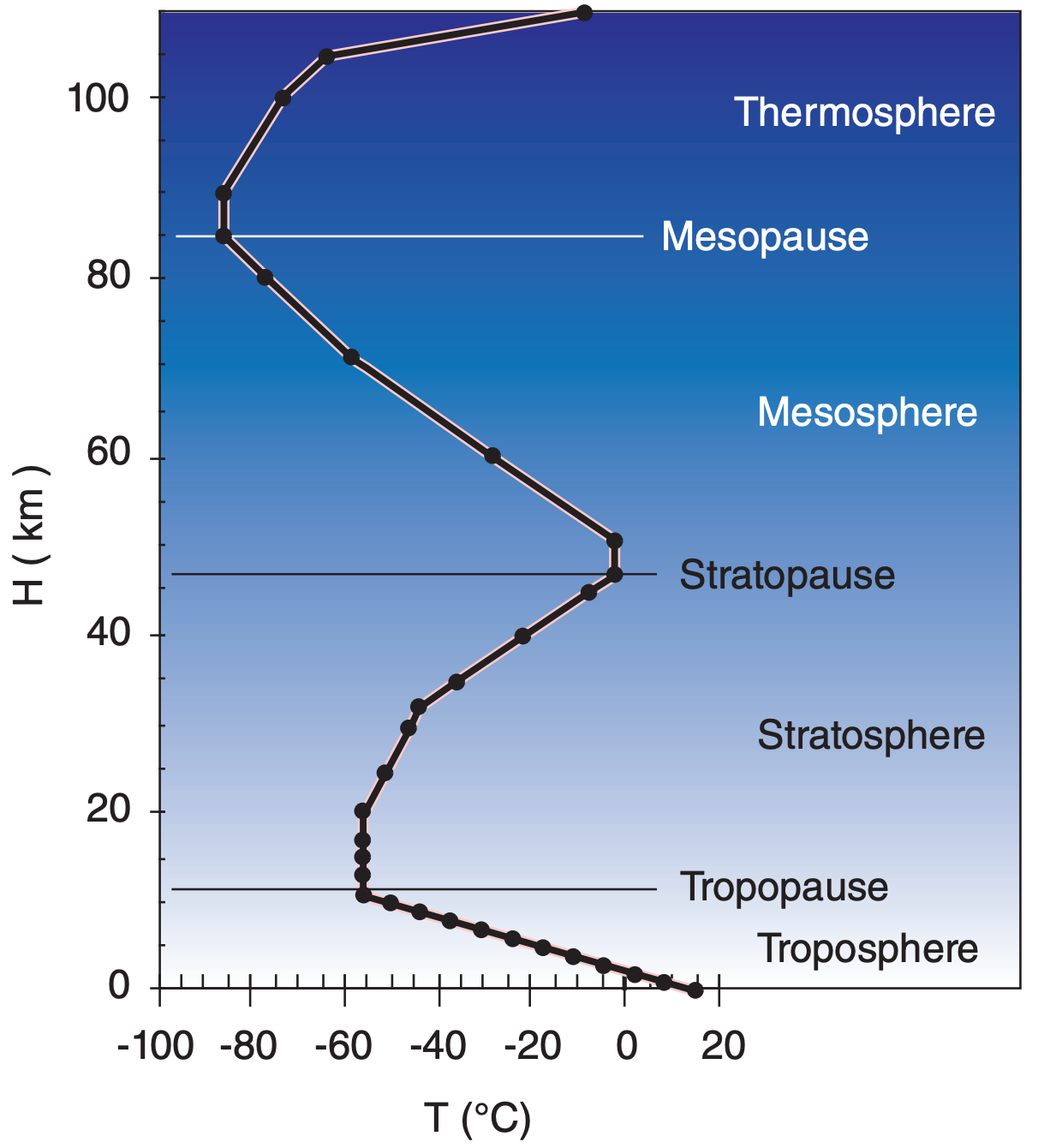
Table 1-5 gives the standard temperature, pressure, and density as a function of geopotential height H above sea level. Temperature variations are linear between key altitudes indicated in boldface. Standard-atmosphere temperature is plotted in Figure 1.10.

Below a geopotential altitude of 51 km, eqs. (1.16) and (1.17) can be used to compute standard temperature and pressure. In these equations, be sure to use absolute temperature as defined by

$\ \begin{align} T(K)=T(^oC)+273.15\tag{1.16}\end{align}$

T = 288.15 K – (6.5 K km^–1)·H	for H ≤ 11 km
T = 216.65 K	11 ≤ H ≤ 20 km
T = 216.65 K +(1 K km^–1)·(H–20km)	20 ≤ H ≤ 32 km
T = 228.65 K +(2.8 K km^–1)·(H–32km)	32 ≤ H ≤ 47 km
T = 270.65 K	47 ≤ H ≤ 51 km

For the pressure equations, the absolute temperature T that appears must be the standard atmosphere temperature from the previous set of equations. In fact, those previous equations can be substituted into the equations below to make them a function of H rather than T. (1.17)

P = (101.325kPa)·(288.15K/T)^–5.255877	H ≤ 11 km
P = (22.632kPa)·exp[–0.1577·(H–11 km)]	11 ≤ H ≤ 20 km
P = (5.4749kPa)·(216.65K/T) ^34.16319	20 ≤ H ≤ 32 km
P = (0.868kPa)·(228.65K/T) ^12.2011	32 ≤ H ≤ 47 km
P = (0.1109kPa)·exp[–0.1262·(H–47 km)]	47 ≤ H ≤ 51 km

These equations are a bit better than eq. (1.9a) because they do not make the unrealistic assumption of uniform temperature with height.

Knowing temperature and pressure, you can calculate density using the ideal gas law eq. (1.18).

Sample Application

Find std. atm. temperature & pressure at H=2.5 km.

Find the Answer

Given: H = 2.5 km. Find: T = ? K, P = ? kPa

Use eq. (1.16): T = 288.15 –(6.5K/km)·(2.5km) = 271.9 K

Use eq. (1.17): P =(101.325kPa)·(288.15K/271.9K)^–5.255877

= (101.325kPa)· 0.737 = 74.7 kPa.

Check: T = –1.1°C. Agrees with Figure 1.10 & Table 1-5.

Table 1-5. Standard atmosphere.
H (km)	T (°C)	P (kPa)	ρ (kg m^–3)
-1 0 1 2 3 4 5 6 7 8 9 10 11 13 15 17 20 25 30 32 35 40 45 47 50 51 60 70 71 80 84.9 89.7 100.4 105 110	21.5 15.0 8.5 2.0 -4.5 -11.0 -17.5 -24.0 -30.5 -37.0 -43.5 -50.0 -56.5 -56.5 -56.5 -56.5 -56.5 -51.5 -46.5 -44.5 -36.1 -22.1 -8.1 -2.5 -2.5 -2.5 -27.7 -55.7 -58.5 -76.5 -86.3 -86.3 -73.6 -55.5 -9.2	113.920 101.325 89.874 79.495 70.108 61.640 54.019 47.181 41.060 35.599 30.742 26.436 22.632 16.510 12.044 8.787 5.475 2.511 1.172 0.868 0.559 0.278 0.143 0.111 0.076 0.067 0.02031 0.00463 0.00396 0.00089 0.00037 0.00015 0.00002 0.00001 0.00001	1.3470 1.2250 1.1116 1.0065 0.9091 0.8191 0.7361 0.6597 0.5895 0.5252 0.4664 0.4127 0.3639 0.2655 0.1937 0.1423 0.0880 0.0395 0.0180 0.0132 0.0082 0.0039 0.0019 0.0014 0.0010 0.00086 0.000288 0.000074 0.000064 0.000015 0.000007 0.000003 0.0000005 0.0000002 0.0000001

1.5.2. Layers of the Atmosphere

The following layers are defined based on the nominal standard-atmosphere temperature structure (Figure 1.10).

Exosphere* Thermosphere Mesosphere Stratosphere Troposphere

(500 to 103) km ≤ z 84.9 ≤ H ≤ (500 to 10^3) km 47 ≤ H ≤ 84.9 km 11 ≤ H ≤ 47 km 0 ≤ H ≤ 11 km

Almost all clouds and weather occur in the troposphere. (*Not defined by the US Standard Atmos. The air is so thin in the exosphere that molecules don’t behave as a gas, and can escape to space.)

The top limits of the bottom three spheres are named:

Thermopause or Exobase Mesopause Stratopause Tropopause

z = 500 - 10^3 km H = 84.9 km H = 47 km H = 11 km

On average, the tropopause is lower (order of 8 km) near the Earth’s poles, and higher (order of 18 km) near the equator. In mid-latitudes, the tropopause height averages about 11 km, but is slightly lower in winter, and higher in summer.

The three relative maxima of temperature are a result of three altitudes where significant amounts of solar radiation are absorbed and converted into heat. Ultraviolet light is absorbed by oxygen and ozone near the stratopause, visible light is absorbed at the ground, and most other radiation is absorbed in the thermosphere.

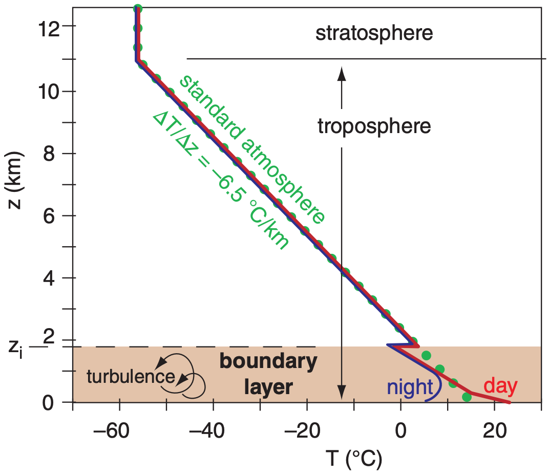
1.5.3. Atmospheric Boundary Layer

The bottom 0.3 to 3 km of the troposphere is called the atmospheric boundary layer (ABL). It is often turbulent, and varies in thickness in space and time (Figure 1.11). It “feels” the effects of the Earth’s surface, which slows the wind due to surface drag, warms the air during daytime and cools it at night, and changes in moisture and pollutant concentration. We spend most of our lives in the ABL. Details are discussed in a later chapter.

Sample Application

Is eq. (1.9a) a good fit to standard atmos. pressure?

Find the Answer

Assumption: Use T = 270 K in eq. (1.9a) because it minimizes pressure errors in the bottom 10 km.

Method: Compare on a graph where the solid line is eq. (1.9a) and the data points are from Table 1-5.

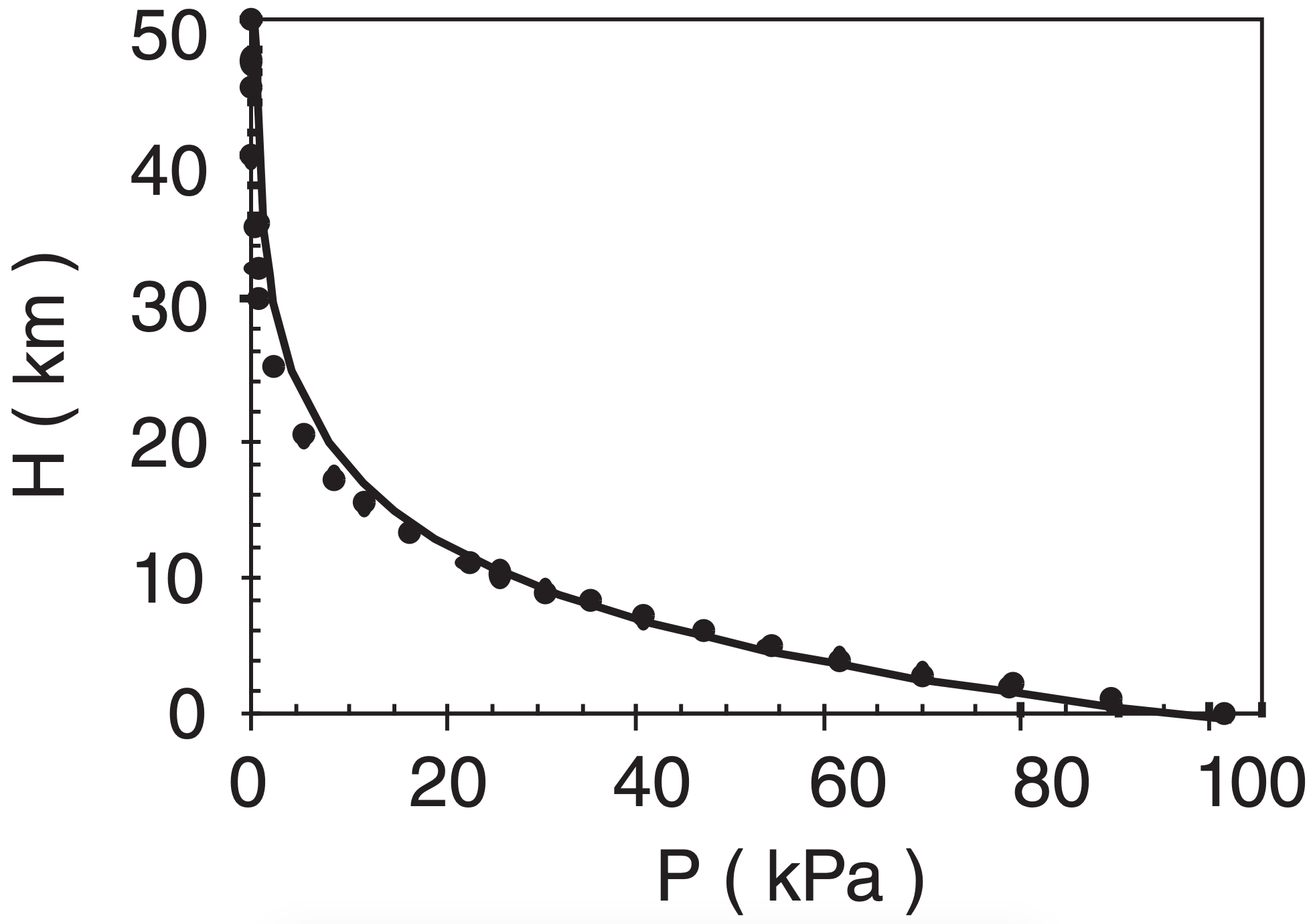
Exposition: Over the lower 10 km, the simple eq. (1.9a) is in error by no more than 1.5 kPa. If more accuracy is needed, then use the hypsometric equation (see eq. 1.26, later in this chapter).

Figure 1.11 Boundary layer (shaded tan) within the bottom of the troposphere. Standard atmosphere is dotted green line. Typical temperature profiles during day (red line) and night (blue line) Boundary-layer top (dashed line) is at height z_i.